EPE and Speed Adaptive Extended Kalman Filter for Vehicle Position
and Attitude Estimation with Low Cost GNSS and IMU Sensors
P. Balzer
1
, T. Trautmann
1
and O. Michler
2
1
Laboratory of Vehicle Mechatronics,
Hochschule f¨ur Technik und Wirtschaft Dresden, Friedrich-List-Platz 1, 01069 Dresden, Germany
2
Chair of Transport Systems Information Technology,
Technische Universit¨at Dresden, Fakult¨at Verkehrswissenschaften ”Friedrich List”, 01062 Dresden, Germany
Keywords:
Multisensor Data Fusion, Adaptive, Extended Kalman Filter, Filter Tuning.
Abstract:
This paper presents a novel approach for an adaptive Extended Kalman Filter (EKF), which is able to han-
dle bad signal quality caused by shading or loss of Doppler Effect for low cost Global Navigation Satellite
System (GNSS) receiver and Inertial Measurement Unit (IMU) sensors fused in a loosely coupled way. It
uses the estimated position error as well as the speed to calculate the standard deviation for the measurement
uncertainty matrix of the Kalman Filter. The filter is very easy to implement, because some conversions of
the measurement, as well as the state variables, are made to reduce the complexity of the Jacobians, which
are used in the EKF filter algorithm. The filter implementation is tested within a simulation and with real data
and shows significantly better performance, compared to a standard EKF. The developed filter is running in
realtime on an embedded device and is able to perform position and attitude estimation of a vehicle with low
cost sensors.
1 INTRODUCTION
The Kalman Filter is widely used in a lot of ap-
plications, since R.E. Kalman introduced it in 1960
(Kalman, 1960). A vast number of papers have been
published about the Kalman Filter and its special vari-
ations for special problems. A lot of them adress-
ing problems about sensor fusion for unmanned au-
tonomous vehicles, e.g. (Penarrocha and Sanchis,
2010; Mourikis and Roumeliotis, 2007; Sun et al.,
2010; Barczyk and Lynch, 2011). Implementations
with adaptive calculation of the measurment uncer-
tainty matrices R and Q are presented, e.g. (Bistrovs
and Kluga, 2012). Some of them deal with different
driving situations (dynamic vs. standing) and using
interactive multimodel fusion filtering, e.g. (Toledo-
Moreo, 2007; Stephen and Lachapelle, 2001). Some
papers addressing problems with low cost sensors,
e.g. (von Rosenberg, 2006; Toledo-Moreo, 2007;
Kingston and Beard, 2004) and odometry to supple-
ment GNSS under signal masking conditions such as
tree foliage and urban canyons, e.g. (Stephen and
Lachapelle, 2001).
Most of the papers using additional sensors like
cameras (Effertz, 2009; von Holt, 2004), wheel rev-
olution sensors (Stephen and Lachapelle, 2001) or
lidar sensors (von Holt, 2004) to get a better posi-
tion estimation. In this paper, we present a novel
and very easy to implement adaptive EKF, which only
uses low cost GNSS sensor and an intertial measure-
ment unit (acceleration, rotation, magnetometer) to
perform very well in dynamic situations and in rest
position of a car.
No additional sensors nor a connection to the ve-
hicle CAN is necessary, which recommends the filter
for portable devices or Smartphones.
2 FUNDAMENTALS
2.1 Kalman Filter
As introduced in (Kalman, 1960), the Bayesian track-
ing algorithm estimates the probability density func-
tion (PDF) of a systems state vector x
k
, recursively. In
one timestep k the system state evolves with the state
transition equation
x
k+1
= g(x
k
,u
k
,ω
k
) (1)
to the next state. The noise ω is assumed to be zero
mean multivariate Gaussian white noise with covari-
649
Balzer P., Trautmann T. and Michler O..
EPE and Speed Adaptive Extended Kalman Filter for Vehicle Position and Attitude Estimation with Low Cost GNSS and IMU Sensors.
DOI: 10.5220/0005023706490656
In Proceedings of the 11th International Conference on Informatics in Control, Automation and Robotics (ICINCO-2014), pages 649-656
ISBN: 978-989-758-039-0
Copyright
c
 2014 SCITEPRESS (Science and Technology Publications, Lda.)

ance Q.
ω
k
∼ W N (0,Q
k
) (2)
The control input u drives the state. The measurement
function
y
k
= h(x
k
,ν
k
) (3)
maps the measurements to the state vector with mea-
surement noise ν, which is as well assumed to be
ν
k
∼ W N (0,R
k
) (4)
with the measurement noise covariance matrix R.
2.2 Uncertainty Matrices
The matrices have different roles in the Kalman Filter.
The matrix Q models the uncertainty, which superim-
pose the system model. The matrix R models the un-
certainty associated with the measurements. The error
covariance matrix P is the matrix, which is recalcu-
lated in the prediction as well as in the correction step,
by the Kalman filter itself. It shows the uncertainty of
the state estimate as a function of time. Therefore, the
values in P should decrease over time.
2.3 Linearization
The Kalman Filter actually just works for linear states
and measurements. Most of real life problems, like
the one presented in this paper, are nonlinear, either
on the dynamic or the measurement, or both. The the-
ory behind is, that a nonlinear state or measurement
can be estimated by a Taylor approximation. The par-
tial derivative of the state and the measurement with
respect to state vector x or control vector u is well
known as the Jacobian.
J
A
=
∂g
∂x




ˆx
k
,u
k
(5)
J
G
=
∂g
∂u




ˆx
k
,u
k
(6)
J
H
=
∂h
∂x




ˆx
k
,u
k
(7)
2.4 Extended Kalman Filter
Both, the Uncented and the Extended Kalman Fil-
ter perform evenly well on nonlinear states, but like
St. Pierre et. al. in (St-Pierre and Gingras, 2004)
pointed out, the Extended Kalman Filter is signifi-
cantly more efficient in computational time. Depend-
ing on the complexity of the state transition function
(1) and measurement function (3), the EKF is up to
22x faster (St-Pierre and Gingras, 2004).
Project the state ahead
x
k+1
= g(x
k
, u)
Project the error covariance ahead
P
k+1
= J
A
P
k
J
A
T
+ J
G
QJ
G
T
Compute the Kalman Gain
K
k
= P
k
J
H
T
(J
H
P
k
J
H
T
+ R)
−1
Update the estimate via measurement
x
k
= x
k
+ K
k
(z
k
− h(x
k
))
Update the error covariance
P
k
= (I − K
k
J
H
)P
k
Initialize R, P, Q once
Prediction
Correction
J are the Jacobians
Figure 1: Extended Kalman Filter Step.
Because the computational time is an important
fact for real time state estimation, the EKF presented
in this paper uses some calculations/conversions be-
fore the EKF itself, to reduce the complexity of the
Jacobians, especially for the measurement function h.
2.5 GNSS Position Accuracy
In this paper, an adaptive extended Kalman Filter
is introduced, which recalculates the measurement
noise uncertainty for the position, based on the esti-
mated position error (EPE), which is calculated by
the GNSS receiver itself.
As (Sharif and Stein, 2004) wrote, “the EPE is a
scalar indicating the precision of the receiver based on
the deviation of the measurements from the mean of
the measurement.”
For this reason, it cannot be used to determine a
bias in the position measurement of the GNSS, but its
relative error.
EPE ∼ HDOP· URA(1σ) (8)
With HDOP as the Horizontal Delution of Preci-
sion and URA as the User Range Accuracy, which is
a quantity that is transmitted in the navigation mes-
sage and that is the predicted (not measured) statisti-
cal ranging accuracy.
3 EXTENDED KALMAN FILTER
FOR CTRV DYNAMIC WITH
ATTITUDE ESTIMATION
The implemented EKF estimates following state vec-
tor x
k
, which is well known as the constant turn rate
and velocity (CTRV) vehicle model plus additionally
roll and pitch estimation:
ICINCO2014-11thInternationalConferenceonInformaticsinControl,AutomationandRobotics
650

x
k
=







x
y
v
ψ
φ
Θ







=







Position x (GNSS)
Position y (GNSS)
Speed (GNSS)
Heading (GNSS)
Pitch (IMU)
Roll (IMU)







(9)
As Schubert et. al. determined in (Schubert et al.,
2011), ”for ego motion estimation purposes which are
characterized by a high update rate and the observ-
ability of v and
˙
ψ, model complexities beyond CTRV
do not appear to be beneficial. However, the CTRV
model shows its advantages as soon as a heading es-
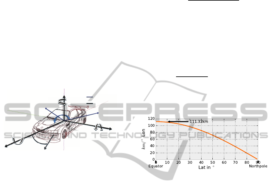
timate is required.” The coordinate system is defined
as shown in Fig. 2.
"#!
"$%&!!
"'()*+!!
",-..!!
"/(012.(3!!
"4!
"5!!
"$!!
"61%0(78!!
8.-9%.!
41+(*.1!:(;10!
Figure 2: Right hand coordinate system with z-axis to top.
3.1 Roll and Pitch Angle
In (Madgwick, 2010), Madgwick presents an efficient
orientation filter for inertial and inertial/magnetic sen-
sor arrays. ”The filter uses a quaternion representa-
tion, allowing accelerometer and magnetometer data
to be used in an analytically derived and optimised
gradient-descent algorithm to compute the direction
of the gyroscope measurement error as a quaternion
derivative.”. The filter is implemented on the IMU
and provides attitude information in quaternion rep-
resentation in the global IMU coordinate system.
As mentioned there, the filter only estimates the
correct attitude, if no external acceleration is actuat-
ing the vehicle. The calculated roll and pitch angles
are actually just valid while standing still, not while
accelerating/braking or cornering.
Madgwick recommended to adaptively choose
convergence parameters, depending on absolute ac-
celeration, influencing the IMU.
This paper lives this recommendation up and in-
troduces an adaptively chosen weighting of roll and
pitch angle, depending on the accelerations in lateral
or longitudinal direction.
The roll and pitch angles, in vehicle coordinate
system, are calculated with the quaternion (Z
D
= a−
bi
1
− ci
2
− di
3
) output of the orientation filter (Buch-
holz, 2013).
φ = − arcsin(2· (a· c− b · d)) (10)
θ = −arctan

2· (c· d + a· b)
−(a
2
− b
2
− c
2
+ d
2
)

(11)
3.2 Position
The position x and y is determined with a low cost
GNSS receiver. The conversion between WGS84 Lat
and Lon decimaldegrees to SI units is calculated as
follows: Assume the earth’s radius at a specific alti-
tude with R = 6378km+ alt, then one degree of Lon
at alt = 0m is
arc =
2π · (R+ alt)
360
◦
= 111,32km/
◦
(12)
One degree Lat is 111,32km only near the equa-
tor. If moving to the poles, the value decreases until it
is 0km on North- or Southpole. Taking the cos of the
Lat provides the correct length reduction (see Fig. 3).
Figure 3: Length of one degree of Longitude, depending on
Latitude (WGS84).
∆x = arc· cos(Lat) · ∆Lon (13)
∆y = arc· ∆Lat (14)
With these equations the distance moved between
two GNSS measurements can be calculated very ac-
curate and additionally they simplify the state transi-
tion equations and the measurement function h, com-
pared to other implementations, e.g. in (Wender,
2008).
3.3 State Control
The longitudinal acceleration a
x
, rollrate
˙
Θ, pitchrate
˙
φ and the yawrate
˙
ψ are state control variables.
u
k
=

a
x
˙
ψ
˙
φ
˙
Θ

T
(15)
They are acquired by the IMU. The proposed fil-
ter could be used without any physical connection to
the vehicle sensors (e.g. CAN-Bus) and therefore it
is useful for mobile measurement systems. The state
control vector u consists only of values, acquired by
the IMU, so the filter can run with high update rate in
dead reckoning mode without GNSS information and
the measurements from GNSS are used with lower
update rate as correction.
EPEandSpeedAdaptiveExtendedKalmanFilterforVehiclePositionandAttitudeEstimationwithLowCostGNSSand
IMUSensors
651

3.4 State Transition Function
The state transition function g(x
k
,u
k
) is defined with
x
k+1
=








x+
v
˙
ψ
(−sin(ψ) + sin(T
˙
ψ+ ψ))
y+
v
˙
ψ
(cos(ψ) − cos(T
˙
ψ+ ψ))
Ta
x
+ v
T
˙
ψ+ ψ
T
˙
φ+ φ
T
˙
Θ+ Θ








(16)
for
˙
ψ 6= 0 and with T as the time between two fil-
tersteps. The Jacobians of the state transition with
respect to the state and w.r.t. the control are listed in
appendix.
3.5 Process Noise Covariance Matrix Q
As Kelly in (Kelly, 1994) pointed out ”a Kalman fil-
ter is a mathematical idealization that happens to be
useful in practice. However, it is important to note
that there is a big difference between an optimal es-
timate and an accurate estimate. In practical use, the
uncertainty estimates take on the significance of rela-
tive weights of state estimates and measurements. So
it is not so much important that uncertainty is abso-
lutely correct as it is that it be relatively consistent
across all models.”
Q = diag
h
σ
2
a
σ
2
˙
ψ
σ
2
˙
φ
σ
2
˙
Θ
i
(17)
Cross covariances resulting from deviation mo-
ments are assumed to be zero.
Assumptions for process noises for a vehicle
model are suggested in (Kelly, 1994). The process
noise is best described with the question, how much
the state can be propagated in one timestep by ex-
pected movement of the vehicle. So the jerk expected
for a car might be 300m/s
3
under normal circum-
stances, so the σ
a
≈ ˙a
max
· T.
A typical maximal angular acceleration around
vehicle z-axis might be 80
◦
/s
2
, which leads to a pro-
cess noise of σ
˙
ψ
≈ 80
◦
/s
2
·
π
180,0
· T. The rotation
around the pitch axis is much more dynamically, with
typical angular accelerations of 200
◦
/s
2
because of
bumps and road surface quality. The angular acceler-
ation around the roll axis is assumed to be 200
◦
/s
2
,
too.
The process noises for a 50Hz filter are listed in
Table 1.
3.6 Measurement Noise Covariance R
The attitude estimation of the IMU filter (Madgwick,
2010), which is used as measurement for roll (10)
Table 1: Process Noise Standard Deviations
Parameter Process Noise for Value
σ
a
Acceleration 6,0m/s
2
σ
˙
ψ
Yawrate 0,028rad/s
σ
˙
φ
Pitchrate 0,070rad/s
σ
˙
Θ
Rollrate 0,070rad/s
and pitch (11), is only valid for quasistatic situations
(which is acutally not valid for a moving vehicle), the
standard deviation for the calculated attitude angles
are adaptive to the accelerations a
x
for pitch and a
y
for roll.
The novel approach, presented in this paper, is the
very easy to implement and fast to calculate elements
of the measurement noise covariance matrix R.
R = diag

σ
2
x
σ
2
y
σ
2
v
σ
2
ψ
σ
2
φ
σ
2
Θ

(18)
The standard deviations are adaptively calculated
as follows.
3.6.1 Position Measurement Uncertainties
In every EKF filterstep, the standard deviations for
σ
x
and σ
y
are calculated, depending on the speed and
additionally dependingon the estimated position error
(EPE), which is provided by the GNSS modul itself.
σ
2
x
= σ
2
y
= c· σ
2
v
+ σ
2
EPE
(19)
with
σ
v
= (v+ ε)
−ξ
(20)
σ
EPE
= ζ· EPE (21)
The variables ε, ξ and ζ are tuneable parameters.
Factor [c] = s
2
for unit correction.
3.6.2 Attitude Measurement Uncertainty
The uncertainty for roll and pitch angle are adaptively
calculated, depending on the vehicle accelerations in
the appropriate directions.
σ
Θ
= (ρ+ γ · a
y
)
2
(22)
σ
ψ
= (ρ+ γ · a
x
)
2
(23)
The variables ρ and γ are tuneable parameters.
3.7 Measurement Function h
Because of the simplifications (13) and (14), the Ja-
cobian of the measurement function h with respect to
the state x
k
is simple and computationally fast with
J
H
= diag

1 1 1 1 1 1

(24)
ICINCO2014-11thInternationalConferenceonInformaticsinControl,AutomationandRobotics
652

when a new GNSS position measurement is available.
In the practical implementation, the GNSS provide
position information with 10,0Hz and the EKF is esti-
mating with 50,0Hz (IMU measurement frequency).
If no GNSS position information is available, the cor-
respondig elements in J
H
are zero.
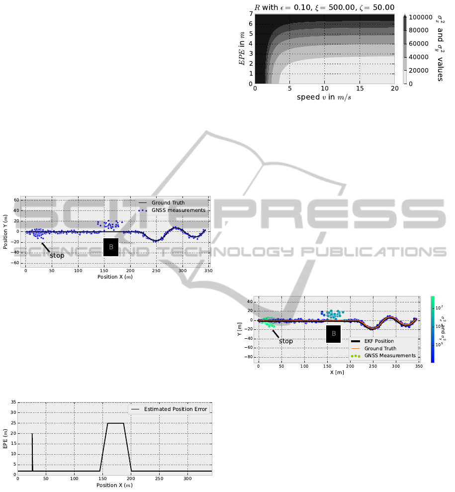
4 SIMULATION
4.1 Simulation Setup
To evaluate the adaptive EKF, a typical urban sce-
nario, with shading from a building, as well as a vehi-
cle stop, was simulated (see Fig. 4).
Figure 4: Simulated GNSS measurements with vehicle stop
and shading from a building (B) as well as ground truth.
The car starts at x = 0, y = 0 with v = 20,0km/h
and decelerates until it stops. It is standing for 10s
and accelerating until it reaches v = 50,0km/h again.
Then it is passing a building, which corruptsthe signal
quality of the GNSS, and the position measurement is
disrupted by +15m in y-direction.
Figure 5: Simulated GNSS Estimated Position Error.
After that, the car performs a slalom maneuvers to
evaluate the dynamic capabilities of the filter.
4.2 Parameter for Adaptive R
The summand ε for (20) is initialized with 0,1m/s,
the exponent ξ for (20) with 500,0 and the factor ζ for
(21) with 50,0. The resulting values for σ
2
x
and σ
2
y
for
a range of velocities and EPEs are shown in Fig. 6.
Figure 6: Values of σ
2
x
and σ
2
y
in R, depending on v and
EPE
The factor ρ for (22) was initialized with 200,0,
the summand γ was chosen to be 500,0.
These parameters are empirically chosen and are
subject to change for different cars or other driving
scenarios or street qualities.
4.3 Simulation Results
As one can see in Fig. 7, the filter follows the trajec-
tory of the GNSS measurements. If the EPE raises,
the filter is more willing to trust the control input in-
stead of the position measurements.
Figure 7: Measurements of GNSS with color coded value
for R, depending on speed and EPE as well as estimated
trajectory of the EKF.
To quantify the filter performance with respect to
ground truth (GT) trajectory, the cross track error is
introduced.
CTE
x
= x
GT
− x (25)
CTE
y
= y
GT
− y (26)
The sum of the square of the CTE over the whole
dataset is a value to quantify the filter performance
with respect to the correct trajectory estimation.
4.4 Comparison to Standard EKF
To compare the estimated trajectory with a non-
adaptiveEKF, the estimation was performedwith sev-
eral datasets for GNSS position measurements, gen-
erated by random Gaussian noise around the ground
truth position.
The standard EKF was set up with static σ
2
x
=
EPEandSpeedAdaptiveExtendedKalmanFilterforVehiclePositionandAttitudeEstimationwithLowCostGNSSand
IMUSensors
653

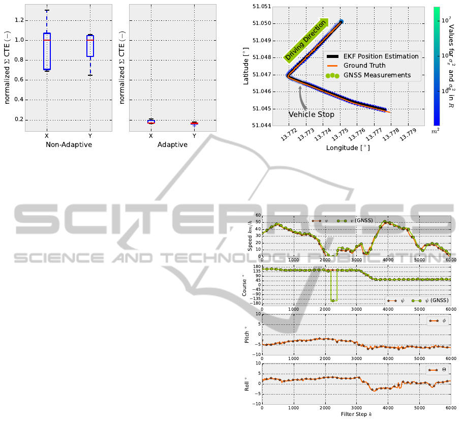
Figure 8: Comparison of the mean, upper and lower quan-
tile of several runs for trajectory estimation and values for
sum of squares of the CTE for the adaptive and the standard
EKF
144m
2
, σ
2
y
= 144m
2
values. The result is shown in
Fig. 8.
In comparison, the adaptive EKF reduces the
ΣCTE
2
x,y
by around 80%, which for sure depends on
the driving direction as well as on the chosen param-
eters.
Note, that the standard EKF could set up with high
values for R as well and may have better CTE values,
but then, like for all filters, the dynamic is getting lost.
5 EXPERIMENTAL SETUP
5.1 Low Cost Sensors
The measurement and control data of the filter were
logged by a LSM303 3-axis accelerometer and 3-
axis magnetometer, ITG-3200 3-axis gyro and PA6H
GNSS receiver. The sensors are available with the
Tinkerforge IMU Brick and GPS Bricklet.
All sensors are mobile, so no connection to the car
is neccessary, but could improve the estimation.
5.2 Ground Truth GNSS Sensor
The ground truth was logged with a multifrequency
aerial antenna (JAVAD GrAnt-G3T) and -receiver
(JAVAD Delta), corrected with a virtual reference sta-
tion (VRS) and Satellite Positioning Service of the
German State Survey (SAPOS) data via GPRS mo-
dem (come2ascos GenPro).
6 EXPERIMENTAL RESULTS
The state variables x
k
for the scenario were estimated
Figure 9: Performed test drive with adaptive values of mea-
surement uncertainty values for matrix R. (GNSS measure-
ment dots are reduced to every 10th for better visualisation
in this figure).
Figure 10: Estimated state variables x
k
for real world test
drive.
as shown in Fig. 10.
As one can see, the stop before the right turn got a
high position measurement uncertainty, which in de-
tail is shown in figure 11.
While standing still, the heading measurement of
the GNSS receiver is inaccurate (see Fig. 10 be-
tween filter step k ≈ 2200. . .2400). The filter per-
formes very well on this situation and keeps the head-
ing in the correct direction. The EKF position es-
timation (see Fig. 11) is not disturbed by inaccu-
rate GNSS measurements while standing still and is
dynamically responsive while cornering. The low
cost GNSS equipment with the proposed adaptive Ex-
tended Kalman Filter delivers a robust position esti-
mation, which alignes with the ground truth measure-
ment.
ICINCO2014-11thInternationalConferenceonInformaticsinControl,AutomationandRobotics
654

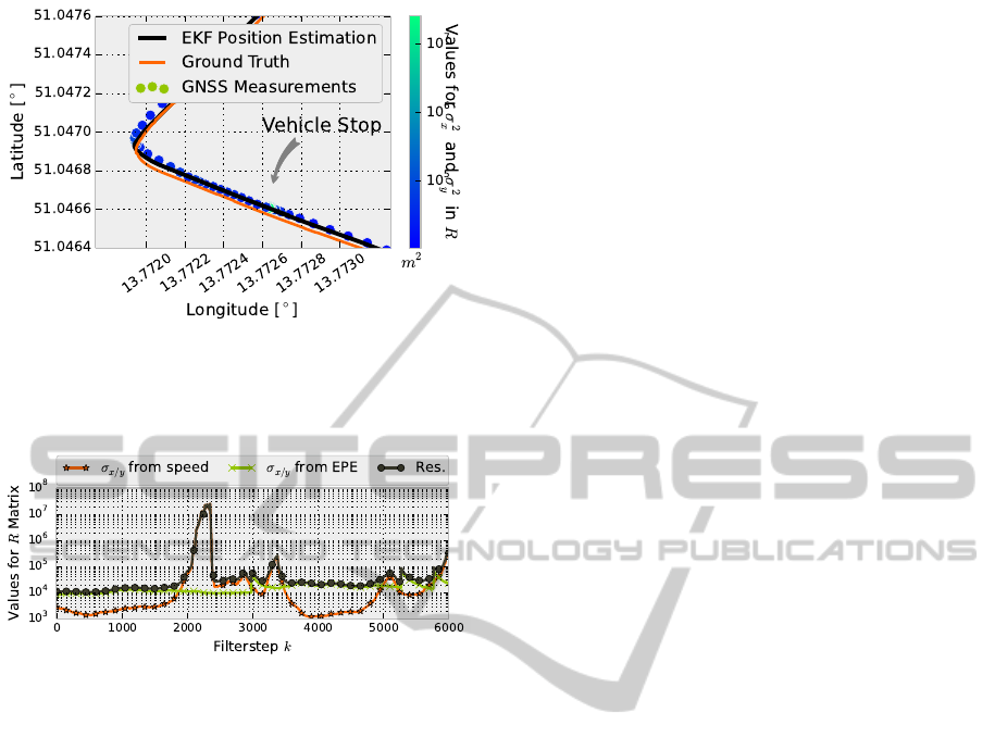
Figure 11: Detailed view of the stop within the performed
test drive with raised uncertainty for R. (GNSS measure-
ment dots are reduced to every 10th for better visualisation
in this figure).
Figure 12: Values for adaptive σ
v
, σ
EPE
and resulting σ for
x and y.
The values for the measurement uncertainties in R
are calculated like shown in figure 12.
7 CONCLUSIONS
In this paper we presented a novel approach to adap-
tively calculate the measurement uncertainty for an
improved position and attitude estimation, based on
the Estimated Position Error and the speed, deter-
mined by the low cost GNSS receiver. We explained
the basics and used some empirically chosen values
to parametrize the filter. With that, we showed with
simulated data, that the filter performes significantly
better than a standard Extended Kalman Filter. Based
on that, we conducted test drives and used the devel-
oped Adaptive EKF for a real world dataset, which
proved its ability to improve the position estimation
with partly bad signal quality. In addition to that, the
filter also performs pretty well on dynamic situations
and is not loosing the ability to follow dynamic vehi-
cle movements. The filter cannot be used to get rid
of bias in position estimation, because the EPE from
GNSS has, by definition, no information about static
drift of the position information. The presented fil-
ter can be used to get significantly better results while
standing still or driving slowly as well as keeping the
heading fixed while do so. Additionally, the attitude
of the vehicle is estimated, based on the filter pre-
sented in (Madgwick, 2010).
ACKNOWLEDGEMENTS
The authors would like to thank the Free State of Sax-
ony and the European Union, which funded this re-
search from the ESF fond.
REFERENCES
Barczyk, M. and Lynch, A. F. (2011). Invariant Extended
Kalman Filter design for a magnetometer-plus-GPS
aided inertial navigation system. IEEE Conference on
Decision and Control and European Control Confer-
ence, pages 5389–5394.
Bistrovs, V. and Kluga, A. (2012). Adaptive Extended
Kalman Filter for Aided Inertial Navigation System.
Electronics & Electrical Engineering, 6(6).
Buchholz, J. J. (2013). Vorlesungsmanuskript Regelung-
stechnik und Flugregler.
Effertz, J. (2009). Autonome Fahrzeugf¨uhrung in urbaner
Umgebung durch Kombination objekt- und karten-
basierter Umfeldmodelle. PhD thesis, Technische
Universit¨at Carolo-Wilhelmina zu Braunschweig.
Kalman, R. E. (1960). A New Approach to Linear Filtering
and Prediction Problems. 82(Series D):35–45.
Kelly, A. (1994). A 3D state space formulation of a naviga-
tion Kalman filter for autonomous vehicles. (May).
Kingston, D. and Beard, R. (2004). Real-Time Attitude and
Position Estimation for Small UAVs Using Low-Cost
Sensors. AIAA 3rd ”Unmanned Unlimited” Technical
Conference, Workshop and Exhibit, pages 1–9.
Madgwick, S. (2010). An efficient orientation filter for in-
ertial and inertial/magnetic sensor arrays. Report x-io
and University of Bristol.
Mourikis, A. and Roumeliotis, S. (2007). A Multi-State
Constraint Kalman Filter for Vision-aided Inertial
Navigation. Proceedings 2007 IEEE International
Conference on Robotics and Automation.
Penarrocha, I. and Sanchis, R. (2010). Adaptive extended
Kalman filter for recursive identification under miss-
ing data. 49th IEEE Conference on Decision and Con-
trol (CDC), pages 1165–1170.
Schubert, R., Adam, C., Obst, M., Mattern, N., Leonhardt,
V., and Wanielik, G. (2011). Empirical evaluation of
vehicular models for ego motion estimation. 2011
IEEE Intelligent Vehicles Symposium (IV), pages 534–
539.
Sharif, M. and Stein, A. (2004). Integrated ap-
proach to predict confidence of GPS measurement.
isprsserv.ifp.uni-stuttgart.de.
EPEandSpeedAdaptiveExtendedKalmanFilterforVehiclePositionandAttitudeEstimationwithLowCostGNSSand
IMUSensors
655

St-Pierre, M. and Gingras, D. (2004). Comparison between
the unscented Kalman filter and the extended Kalman
filter for the position estimation module of an inte-
grated navigation information system. Intelligent Ve-
hicles Symposium, 2004 ... .
Stephen, J. and Lachapelle, G. (2001). Development
and Testing of a GPS-Augmented Multi-Sensor Ve-
hicle navigation system. The Journal of Navigation,
54:297–319.
Sun, F. S. F., Xu, W. X. W., and Li, J. L. J. (2010). Enhance-
ment of the Aided Inertial Navigation System for an
AUV via micronavigation. OCEANS 2010.
Toledo-Moreo, R. (2007). High-integrity IMM-EKF-
based road vehicle navigation with low-cost
GPS/SBAS/INS. Intelligent .. . , 8(3):491–511.
von Holt, V. (2004). Integrale multisensorielle Fahrumge-
bungserfassung nach dem 4D-Ansatz. PhD thesis,
Universit¨at der Bundeswehr M¨unchen.
von Rosenberg, H. (2006). Sensorfusion zur Navigation
eines Fahrzeugs mit low-cost Inertialsensorik. Diplo-
marbeit, Universit¨at Stuttgart.
Wender, S. (2008). Multisensorsystem zur erweiterten
Fahrzeugumfelderfassung.
APPENDIX
Programm Code and EKF
Implementation
The implemenented EKF code as well as all figures
and the data used in this paper can be found online at
https://github.com/balzer82/ICINCO-2014
Jacobians
The Jacobian of the state transition function (16) with
respect to the state x
k
is defined with







1 0 J
A,13
J
A,14
0 0
0 1 J
A,23
J
A,24
0 0
0 0 1 0 0 0
0 0 0 1 0 0
0 0 0 0 1 0
0 0 0 0 0 1







(27)
with
J
A,13
=
1
˙
ψ
(−sin(ψ) + sin(T
˙
ψ+ ψ)) (28)
J
A,14
=
v
˙
ψ
(−cos(ψ) + cos(T
˙
ψ+ ψ)) (29)
J
A,23
=
1
˙
ψ
(cos(ψ) − cos(T
˙
ψ+ ψ)) (30)
J
A,24
=
v
˙
ψ
(−sin(ψ) + sin(T
˙
ψ+ ψ)) (31)
The Jacobian of the state transition function with
respect to the control is
J
G
=







0 J
G,12
0 0
0 J
G,22
0 0
T 0 0 0
0 T 0 0
0 0 T 0
0 0 0 T







(32)
with
J
G,12
=
Tv
˙
ψ
cos(T
˙
ψ+ ψ)−
v
˙
ψ
2
(−sin(ψ) + sin(T
˙
ψ+ ψ))
(33)
J
G,22
=
Tv
˙
ψ
sin(T
˙
ψ+ ψ)−
v
˙
ψ
2
(cos(ψ) − cos(T
˙
ψ+ ψ))
(34)
ICINCO2014-11thInternationalConferenceonInformaticsinControl,AutomationandRobotics
656