Multi-loop Control Using Gershgorin and Ostrowski Bands

C. Le Brun

, E. Godoy

, D. Beauvois

, N. Doncque

and R. Noguera

Automatic Control Department, Supelec, Gif-sur-Yvette, France

Systems Division, SNECMA (SAFRAN), Villaroche, France

DynFluid Laboratory, Arts & Métiers ParisTech, Paris, France

Keywords: Multivariable Control, Decentralized Control, PID Tuning, Nyquist-Array Methods, Gershgorin Bands,

Ostrowski Bands, Diagonal Dominance.

Abstract: The goal of this paper is to develop a new method of decentralized control tuning. This method is based on

Nyquist-Arrays and independently designs monovariable controllers for each loop of the plant while

ensuring the robust stability of the multivariable system. It works on the optimization of a frequency

criterion using the controller’s design parameters. PID controllers have been chosen in this study because of

their good performances for most applications. Finally, the proposed method allows to achieve good

performances and the stability is ensured thanks to the analysis of Gershgorin and Ostrowski bands.

1 INTRODUCTION

The design of the control of a multivariable process

can be achieved with two strategies. The centralized

strategy consists in designing one full MIMO

(Multiple Inputs Multiple Outputs) controller for the

whole system. The different techniques of this

strategy (Skogestad and Postlethwaite, 1996),

including state-feedback, model predictive control,

H-infinity loop-shaping… are usually efficient and

achieve good performances. However, these

methods need a precise enough model, and the

obtained controllers are usually of high-order. The

decentralized strategy consists in dividing the

MIMO process into a combination of several SISO

(Single Input Single Output) processes and to design

mono-loop controllers in order to control the MIMO

process (Albertos and Sala, 2004).

Compared to the centralized strategy, the

decentralized one provides flexibility and needs

fewer parameters to tune, while it is easier to

implement and increases the loop failure tolerance of

closed loop systems. Because of these benefits,

decentralized controllers have been widely used and

different types of methods have been developed as

described in (Huang et al., 2003).

Independent design method (Skogestad and

Morari, 1989) is chosen in this paper, which means

that each loop is designed independently from the

others. The Nyquist array techniques have shown

themselves to be well-suited for practical design of

controllers for multivariable interacting processes

(Garcia, Karimi and Longchamp, 2005), (Chen and

Seborg, 2002).

This paper proposes a new method based on

Nyquist-Arrays. The goal is to design SISO

controllers for any multivariable process (unstable

poles, unstable zeros, dead time) with medium

interactions. Two alternatives are under discussion,

the first one uses Gershgorin bands whereas the

second one uses Ostrowski bands. The study is

limited to PID controllers but it can easily be

generalized.

This paper is organized as follows: Section 2

surveys theoretical preliminaries about the Nyquist-

array methods. Section 3 presents the design of the

control laws and Section 4 exposes simulation

results that demonstrate the efficiency of this

method. Conclusions are presented in Section 5.

2 NYQUIST-ARRAY METHODS

The proposed method is based on the Nyquist-array

methods (Leigh, 1982), (Rosenbrock, 1969), in

which the design of the controller is divided into two

steps. The first one consists in reducing the

interactions in the system so that each control loop

635

Le Brun C., Godoy E., Beauvois D., Doncque N. and Noguera R..

Multi-loop Control Using Gershgorin and Ostrowski Bands.

DOI: 10.5220/0005017406350642

In Proceedings of the 11th International Conference on Informatics in Control, Automation and Robotics (ICINCO-2014), pages 635-642

ISBN: 978-989-758-039-0

 2014 SCITEPRESS (Science and Technology Publications, Lda.)

can be closed separately and independently from the

remaining loops. In the second step, controllers of

the different loops are designed.

This paper focuses on the design of the

controllers but a short summary of the general

methods is recalled.

2.1 Diagonal Dominance

The design of the control laws often requires the

diagonal dominance of the system. A p×p matrix Z

is called row (respectively column) diagonally

dominant if it satisfies (1) (respectively (2)):

ijj

ijiii

ZZRrZ ,...,1,)(

≠,1









(1)

ijj

jiiii

ZZRcZ ,...,1,)(

≠,1









(2)

If the frequency response matrix of a MIMO

system is row (respectively column) diagonal

dominant for the whole frequency domain, it means

that each output is mainly determined by its

corresponding input (respectively each input

determines mainly its corresponding output).

Furthermore, it is clear that a higher degree of

diagonal dominance yields a smaller difference

between the MIMO performance and the

performance of the SISO designs.

2.2 Principe of Nyquist-Array Methods

Nyquist-array methods are divided into two classes:

the Direct Nyquist-Array (DNA) and the Inverse

Nyquist-Array (INA). Both methods have identical

design objectives and the method proposed here can

be applied both with DNA and INA.

Consider a MIMO plant G. The open-loop

transfer matrix Q described in (3) is used in DNA

whereas the inverse of the open-loop is considered

in INA. The structure of the control laws is

described by (4).

)()()( sKsGsQ 

(3)

)()()( sKsKKsK

cba



(4)

is a constant matrix that permutes rows or

columns to reorder the outputs or inputs. It can be

used to avoid unstable off-diagonal elements. K

used to achieve diagonal dominance. An overview

of the methods to find these matrices is found in

(Vaes, 2005) and (Maciejowski, 1989). K

is a

diagonal matrix composed of separate SISO

controllers for each loop.

In DNA, the diagonal matrix K

post-multiplies

the plant G

as in (5). The effect of each element is

to multiply each column of G

by the same transfer

function. Hence, column dominance of G

preserved.

However, in the INA, K

-1

pre-multiplies the

inverse of the plant and row dominance of the

inverse is conserved.

)()()( sKsGsQ



(5)

)()()( sKKsGsG

bad



(6)

This paper focuses on the design of the diagonal

controller K

only. Therefore, G

is considered as

being column diagonally dominant when working

with DNA and G

-1

is considered as being row

diagonally dominant when working with INA in the

following.

2.2.1 Direct Nyquist-Array Method

Closed-loop stability of a SISO system is obviously

analyzed with the Nyquist stability theorem. The

Generalized Nyquist theorem extends it to MIMO

systems (Macfarlane and Postlethwaite, 1977):

Considering an open loop transfer matrix Q

presenting n

pol

unstable poles, defining the

characteristic loci as the images of the Nyquist

contour by the eigenvalues of Q, the Generalized

Nyquist theorem states that the closed loop is stable

if and only if the sum of the anticlockwise

encirclements around the critical point of the

characteristic loci of the open-loop transfer equals

pol

The characteristic loci can be approached by the

diagonal elements of Q thanks to Gershgorin’s

theorem:

The eigenvalues of a complex p×p matrix Z lie in

the union of the p circles, each with center Z

and

radius Rr or Rc defined in (1) and (2). When this

theorem is applied to the gain matrix Q(jω), a circle

is obtained around each diagonal element of the loop

gain at each frequency ω. The bands obtained by

taking these circles together over the frequency

domain are called Gershgorin bands.

Using Gershgorin's theorem, it can be claimed

that the eigenvalues of a gain matrix Q over all

frequencies are trapped into these Gershgorin’s

bands. Based on the generalized Nyquist theorem, it

can be concluded that if all Gershgorin bands

exclude the critical point, then closed-loop stability

can be assessed by counting the number of

encirclements of the critical point by the Gershgorin

bands.

The open-loop matrix in (5) can be written:

ICINCO2014-11thInternationalConferenceonInformaticsinControl,AutomationandRobotics

636















pppp

KGKG







1111

(7)

The width of the i

column Gershgorin band is:







ikk

ikii

jKjGjRc

)()()(



(8)

It is clear that the width of this band only

depends on the system and on the i

controller K

The stability of the i

loop can thus be ensured

independently of the other controllers.

2.2.2 Inverse Nyquist-Array Method

The principle of the INA (Bell, Cook, and Munro,

1982) method is different. For notational

convenience, the inverse of a matrix H is noted as Ĥ.

Let us consider Q an open-loop transfer matrix

composed of a plant and its SISO controllers as

described in (5) and H the closed-loop transfer

matrix. We denote l

the open-loop transfer function

between e

and y

with all the other loops are closed

as shown in Figure 1 for a TITO (Two Inputs Two

Outputs) process.

Figure 1: TITO process (the second loop is closed and the

first one is being closed).

Considering this open-loop transfer function l

takes into account the stability of the whole system.

is not a priori known but ܳ

෠

௜௜

gives a good

approximation of the inverse of l

thanks to

Ostrowski’s theorem: Considering a complex p×p

matrix Z diagonally row dominant, then:





















∑∑

≠1≠1

max1

jk,k

jjjk

ik,k

ikiiii

ZZZZ

(9)

Applying this theorem to the i

row of Ĥ that is

supposed row diagonally dominant, we obtain after

calculation:

)())(

()(1)(



jjQRrjljQ

iiiii



(10)

))(

(()( max



jQjQRrj

jjj





(11)

Consequently, 1/l

(jω) is contained within a

circle centered in

෠

௜௜

ሺ݆߱ሻ. We call this an Ostrowski

circle and the union of all these circles an Ostrowski

band.

The terms Φ

physically represent the maximal

relative couplings in the other loops. Since ܳ

෠

assumed to be row diagonally dominant, Φ

smaller than 1. The i

Ostrowski band is thus

contained within the i

Gershgorin band of the

inverse of the open-loop transfer matrix. Moreover,

although each term of Φ

depends on the controllers

of the other loops, Φ

is independent of these. It can

be concluded that the width of row Ostrowski bands

only depends on the plant and on the i

controller.

The stability of loop i can thus be ensured

independently of the other loops’ controllers.

As in DNA with Gershgorin bands, Ostrowski

bands can be used to characterize the stability of the

system in INA. The inverse Nyquist criterion (Bell,

Cook, and Munro, 1982) is then used: A feedback

loop with n

zeros

unstable zeros in the loop gain Q is

stable if and only if the sum of the anticlockwise

encirclements around the critical point of the inverse

Nyquist locus of Q equals n

zeros

3 CONTROL LAWS DESIGN

The goal is to define a method to design a

decentralized control for MIMO systems. There is

no restriction about the structure of the controller.

PID controllers have been chosen in this study

because they remain the industry standard and reach

good performances for most applications with an

easy to understand structure. Nevertheless, it is easy

to implement other controller structures in the

algorithm.

The method consists in tuning SISO controllers

independently for each SISO system thanks to the

optimization of a cost function depending on the

controllers parameters. Similar criteria are defined

thereafter for each loop of the system for DNA and

INA analysis.

3.1 Stability

As seen before, to ensure stability, Gershgorin

(respectively Ostrowski) bands must not include the

critical point. Moreover, the bands have to encircle

anticlockwise the critical point a number of times

corresponding to the number of open-loop unstable

poles (respectively unstable zeros).

To take in consideration the number of

encirclements, one idea is to force the Nyquist locus

(respectively the inverse of the Nyquist locus) to

travel through specific areas. After a brief study of

Multi-loopControlUsingGershgorinandOstrowskiBands

637

the plant and the shape of its Nyquist locus, it is

possible to define attractive areas depending on the

number of the open-loop unstable poles

(respectively unstable zeros).

For instance, let us consider an open-loop

monovariable system Q with an unstable pole, the

Nyquist locus of which presents infinite branches

that do not encircle the critical point. Ensuring that

locus crosses the real axis at the left of the critical

point and travelling below it are sufficient conditions

to have closed-loop stability as in Figure 2.

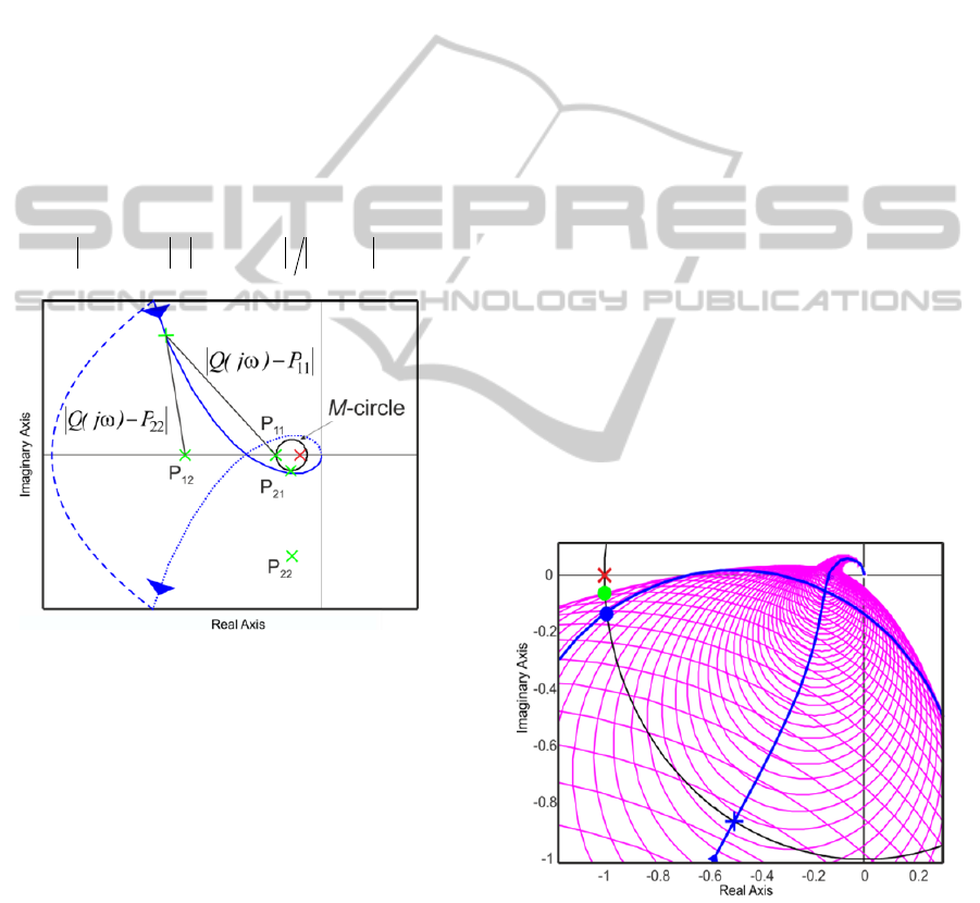
For each attractive area k, a measure of distance

between the nearest point of the Nyquist locus with

the segment [P

] is constituted by (12). To force

the Nyquist locus to travel through these attractive

areas, the distances D

will be minimized. In Figure

2, two attractive areas are defined with [P

] and

]. To facilitate the readability, only the

calculation of D

is presented.

2121

-)-)(-)((inf

kkkkk

PPPjQPjQD







(12)

Figure 2: Calculation of D

with checkpoints P

, and P

This allows to find a controller that stabilizes the

closed-loop system, even if the initial conditions of

the optimization match with a controller

configuration leading to an unstable closed-loop.

For SISO systems, robustness against model

uncertainties is ensured if the direct or inverse

Nyquist loci present sufficient phase margin. Note

that the phase margin of the inverse of a SISO

system is the opposite of the phase margin of the

system.

The determination of the phase margin of a

MIMO system is not obvious (Ye et al., 2008). In

this paper, phase margin is assessed applying the

previous considerations for SISO systems to

Gershgorin bands (respectively Ostrowski bands). In

(Ho, Lee, and Gan, 1997), the circle at the cutoff

frequency is used to determine the phase margin.

The problem is that in some configurations, circles

at other frequencies can be closer from the critical

point than the one at the cutoff frequency.

An example is presented in Figure 3 where the

blue point represents the crossing of the circle at the

cutoff frequency with the unit circle, and the green

point corresponds to the point associated with true

phase margin. Thus, it seems more relevant to

consider the envelope of the circles.

It is then possible to define an objective with a

specified phase margin M

* (when using INA, the

opposite of the specified phase margin is used).

Besides ensuring stability, the phase margin leads to

an upper bound for the damping of the system. It is

also possible to define the gain margin using the

envelope of the bands in the same way. Thus, a

minimum gain margin can be obtained considering a

specified gain margin M

* in the criterion to

optimize (when using INA, the opposite of the

specified gain margin is used).

In DNA, Gershgorin bands ensure the same

stability margins for all loops. Indeed, when the

bands are superimposed (which is often the case

when approaching the critical point), the

characteristic loci of each diagonal element are not

necessarily contained in the Gershgorin bands of this

element. The global stability margins finally match

with the worst stability margins determined from the

different bands.

By contrast, Ostrowski bands can ensure

different stability margins for each loop.

Figure 3: Phase margin for a MIMO process.

3.2 Performances

To give an upper bound of the peak modulus of the

closed-loop frequency response of system, the

complementary modulus margin is considered

ICINCO2014-11thInternationalConferenceonInformaticsinControl,AutomationandRobotics

638

(Bourlès, 2010). It represents physically the inverse

of this maximum gain.

)()(

)()(1

inf





jGdjK





(13)

A criterion is then defined with an objective M

to reach. This specification can be directly

interpreted in the Nyquist diagram thanks to M-

circles (Mirkin, 2011) which are the contours of the

constant closed-loop magnitude. M-circles are

described by the equation:

)²1²(

1²

)(





(14)

X and Y are the real and imaginary coordinates in

the complex plane and M is the magnitude of the

closed-loop transfer function. In order to satisfy

simultaneously stability and closed loop maximum

modulus conditions, the points P

can be chosen

adequately on the specified M-circle as shown in

Figure 2. There are no real rules to set the points P

they only have to be far enough from the points P

The crossover frequency highly impacts the

bandwidth of the closed-loop system. It is then

useful to take it into account in a criterion, defined

with a desired crossover frequency ω

In order to cancel the static error and reduce the

tracking error, the integral action of the controller,

whose structure is given in (15), is maximized:















1

1)(

KsK

(15)

The criteria for previously considered concepts,

are summarized here:





(16)

)(



MMMJ 

(17)

)(

ggg

MMMJ 

(18)

4 ccc

MMMJ 

(19)

5 ccc





(20)

TJ 

(21)

3.3 Optimization

For each SISO loop, the controller parameters are

determined by solving a least-square optimization

problem characterized by a criterion J taking into

account the criteria previously described:





JqJ

(22)

This cost function presents weighting factors q

that give more or less importance to each criterion.

If the initial choice for the parameters lead to a

stable closed-loop system, J

is not necessary. Often,

it is sufficient to take into account J

for robustness

stability so that J

may not be considered. To speed

up the optimization, controllers found with classical

SISO methods (Astrôm and Hägglund, 1995) can be

used for initial conditions.

Each optimization gives the controller parameter

settings for one SISO loop and the tuning of the

other SISO loops do not affect the stability of the

loop already tuned, which makes this method

interesting.

3.4 DNA and INA

As seen in the previous part, the two approaches

work with a similar algorithm. However, conditions

for stability are not the same and the algorithm lead

to different solutions. It is not obvious to guess a

priori which one is the least conservative. The size

of Gershgorin bands of the plant only depends on the

magnitude of the coupling terms. The ratio between

off-diagonal terms and diagonal terms gives the

distance between the bands and the origin of the

Nyquist diagram. However, we are interested in the

distance between the bands and the critical point and

there is no information about that. That is why it is

difficult to know which method to prefer.

Even if the Gershgorin bands can be used to

predict stability when the gains in all the loops

change simultaneously, the DNA method deals with

eigenvalues of the system that can be sensitive to

model perturbations. It is thus less robust than the

INA method where stability is ensured considering a

monovariable system. Another advantage of INA is

that it can be used to indicate whether the system

would be stable if one loop failed.

Finally, the choice of the method is determined

by the shape of the frequency response of the plant.

Ability to make the direct (inverse) open loop

matrix transfer column (row) diagonal dominant can

lead the choice for the method DNA (INA).

3.5 Case of TITO Plants

The case of TITO processes is specific because of

the form of the inverse of the system:































1121

1222

21122211

2221

1211

GGGG

(23)

Multi-loopControlUsingGershgorinandOstrowskiBands

639

If G

is column diagonally dominant, it implies

that G

-1

is row diagonally dominant. In addition, the

ratio between magnitudes of diagonal terms with

off-diagonal terms is conserved.

The consequence is that DNA and INA are not

exclusive. Indeed, the first one requires the column

diagonal dominance of the system and the second

one requires the row diagonal dominance of the

inverse of the system, and these properties are

equivalent. These considerations are only true for

TITO systems. Indeed, in the general case, the

inverse of a column diagonally dominant system is

not a priori row diagonally dominant.

4 SIMULATION EXEMPLES

Academic examples are now considered to

demonstrate the efficiency of this method with a

great variety of processes.

4.1 Optimization with INA

In this first example, G

is a TITO plant described

by:

























)1.06.0(

)5(2.0

)1)(2(

)3.0)(5.0(

)25.0)(4.0(

)1.0(

ssss

(24)

Technical specifications are described in Table 1.

The inverse of the plant is row diagonal dominant,

the INA can thus be applied. Settings of the

designed controller are presented in Table 2. Due to

its negligible derivative action, the first controller

has been simplified in a PI one.

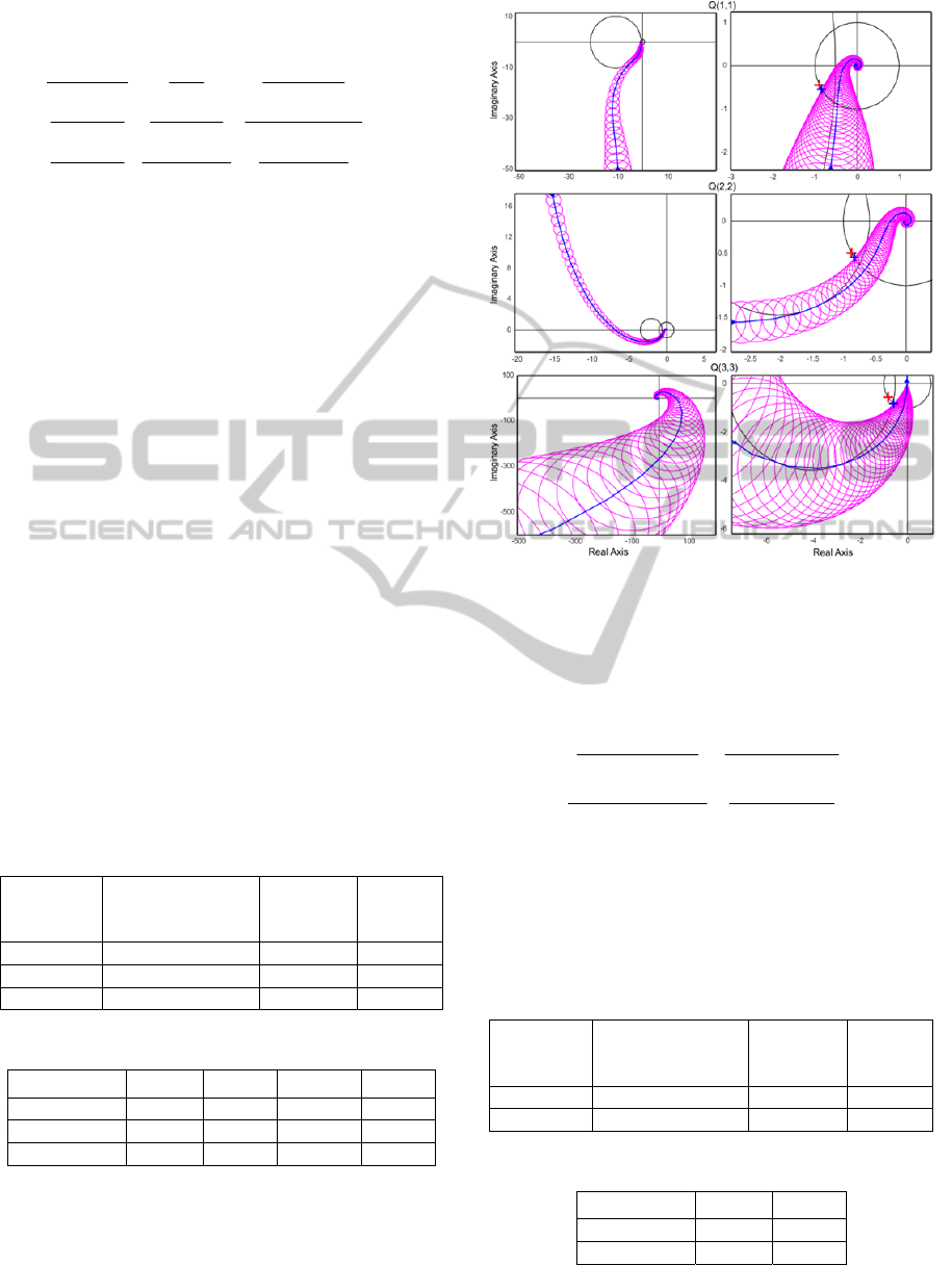
Hereafter figures present Nyquist loci and

inverse Nyquist loci respectively in blue and green,

and the points defining phase margins represented

by crosses. Gershgorin and Ostrowski bands are

respectively drawn in magenta and yellow. Nyquist

diagrams and Gershgorin bands are plotted in Figure

4 for the two diagonal terms. The plots on the left-

hand side give an overview of the Nyquist diagrams.

Table 1: Technical specifications.

Controller

Complementary

Modulus Margin

Crossover

frequency

(rad/s)

Phase

Margin

(°)

1/1.05 0.7 35

Table 2: Controllers parameters.

Controller

0.26 0.47 X X

-0.62 4.2 1.0 33

In the first case, the inverse Nyquist locus and

Ostrowski bands do not encircle the critical point. In

the second loop, the inverse Nyquist locus encircles

the critical point once that is logical because the

second loop contains one unstable zero.

Stability can also be analyzed with Gershgorin

bands. The open-loop transfer matrix is stable and it

can be checked that Gershgorin bands do not

encircle the critical point.

The right diagrams zoom on the critical point to

check that specifications are satisfied. As it can be

seen, phase margins are compliant. For the first loop,

the phase margin obtained with Gershgorin bands is

similar to the one obtained with Ostrowski ones.

However, for the second loop, the phase margin

obtained with Gershgorin bands is clearly smaller

than the one obtained with Ostrowski bands. If DNA

had been chosen, the settings of the controller would

not have been found because the phase margin

would not have been satisfied. The benefits of INA

appear clearly in this case.

M-circles are also drawn to visualize the

complementary modulus margins. For each loop, the

Nyquist loci tangent the M-circles. That means the

complementary modulus margins are fulfilled.

Figure 4: Nyquist-array of the designed loops.

4.2 Optimization with DNA

Consider the MIMO process described by the 3×3

transfer matrix G

in (25). By analysing the plant, it

ICINCO2014-11thInternationalConferenceonInformaticsinControl,AutomationandRobotics

640

can be seen that medium interactions are still

present.







































)5)(20(

)10(3

)15)(50(

)20(5.0

)1)(2(

5.0

)106)(2(

)10(2.0

)05.0exp(

)1)(2(

5.0

)2)(15(

25.0

234

)05.

0exp(8

sss

(25)

To present several study cases, each diagonal

element has a different structure. The first diagonal

term is stable and includes a time delay. The second

diagonal term has one unstable pole and includes a

time delay as well. The third diagonal term includes

an integrator and has two unstable poles.

is column diagonally dominant, the algorithm

with DNA can thus be applied and PID controllers

have been chosen. Technical specifications are

described in Table 3 and details of the controller

settings K

, K

and K

are presented in Table 4.

Due to its negligible derivation action, a PI

controller has finally been designed for the second

loop. Performances broadly match with technical

specifications. Nyquist diagrams and Gershgorin

bands are plotted in Figure 5 for each diagonal term.

As in the first example, the plots on the left-hand

side give an overview of the Nyquist diagrams to

check that the number of anticlockwise

encirclements matches with the number of unstable

poles (respectively 0, 1 and 2 for the three loops). It

can be seen on the diagrams on the right-hand side

that Gershgorin bands do not include the critical

point and fulfilled the specified phase margins.

Moreover, complementary modulus margins are

satisfied.

Table 3: Technical specifications.

Controller

Complementary

Modulus Margin

Crossover

frequency

(rad/s)

Phase

Margin

(°)

1/1.05 10 30

1/1.4 10 30

1/1.15 300 30

Table 4: Controllers parameters.

Controller

4.6 1.1 1 9960

7.45 0.63 X X

1610 0.38 0.065 990

Figure 5: Nyquist-array of the designed loops.

4.3 Analysis using Row and Column

Dominance

Consider now the TITO process:



























)5)(20(

240

)50()100(

)75(100000

)2)(25(

)1.0(30

182580

)1.0exp(2000

(26)

The system is column diagonal dominant and

technical specifications are given in Table 5. The

design is performed with PI controllers with the

proposed algorithm for DNA and details of the

controller settings are presented in Table 6.

Table 5: Technical specifications.

Controller

Complementary

Modulus Margin

Crossover

frequency

(rad/s)

Phase

Margin

(°)

1/1.05 6 45

Table 6: Controllers parameters.

Controller

0.27 0.05

0.54 0.14

In figure 6, Nyquist diagrams of the two diagonal

Multi-loopControlUsingGershgorinandOstrowskiBands

641

elements are plotted in blue and red and the

associated bands are respectively in magenta and

cyan.

Considering column Gershgorin bands in Figure

6a, the worst phase margin does not satisfy the

specified one. It can be noted that Q

is much

smaller than Q

close to the cutoff frequency (bands

of the second loop are much thinner than those of

the first one). By plotting row instead of column

Gershgorin bands as in Figure 6b, the largest bands

become further from the critical point. Thanks to this

analysis, it is possible to ensure the specified phase

margin for the MIMO system.

(a) (b)

Figure 6: Nyquist-array of the designed loops.

Row Gershgorin bands can not be considered for

the design of the controllers as seen before but can

be used to assess stability as well. It is similar for

column Ostrowski bands.

Moreover, once design has been done whatever

the chosen approach, Gershgorin and Ostrowski

bands can be superimposed to determine stability

margins.

5 CONCLUSIONS

This paper proposes a new method of tuning multi-

loop controllers. SISO controllers can be designed

independently using DNA or INA thanks to the

optimization of similar cost functions. The described

procedure aims to reach some performances while

ensuring stability robustness of the closed-loop

multivariable process thanks to Gershgorin bands in

DNA and Ostrowski bands in INA. By

superimposing both Gershgorin and Ostrowski

bands, it is possible in some cases to reduce the

conservatism of the chosen approach.

PID controllers have been chosen in this study

but the method can be easily applied with other

types of controllers.

To conclude, the proposed method offers a

straightforward and systematic way of designing

MIMO controllers, while still leaving freedom to the

designer. Simulation results illustrate the good

performances obtained by this method for a wide

range of processes.

Future works will focus on the adaptation of the

methodology to improve the multivariable

performances, particularly concerning the dynamic

couplings of the closed-loop system.

REFERENCES

Albertos, P., Sala, A., 2004. Multivariable control

systems. Springer.

Aström, K., Hägglund, T., 1995. PID Controllers: Theory,

Design, and Tuning, 2

edition, ISA.

Bell, D. J., Cook, P. A., Munro N., 1982. Design of

Modern Control Systems. Peter Peregrinus.

Bourlès, H., 2010. Linear Systems. Wiley.

Chen, D., Seborg, D. E., 2002. “Multiloop PI/PID

controller design based on Gershgorin bands”. IEEE

Proceedings, Control Theory and Applications.

Garcia, D., Karimi, A., Longchamp, R., 2005. “PID

Controller Design for Multivariable Systems using

Gershgorin Bands”. IFAC.

Ho, W. K., Lee, T. H., and Gan, O. P., 1997. “Tuning of

multiloop PID controllers based on gain and phase

margin specifications”. Industrial & Engineering

Chemistry Research.

Huang, H. P., Jeng, J. C., Chiang, C. H., Pan, W., 2003.

“A direct method for multi-loop PI/PID controller

design”. Journal of Process Control 13, 769-786.

Leigh, J. R., 1982. Applied Control Theory. Peter

Peregrinus.

Macfarlane, A. G. J., Postlethwaite, I., 1977. “The

Generalized Nyquist Stability Criterion and

Multivariable Root Loci”. International Journal of

Control.

Maciejowski, J. M., 1989. Multivariable Feedback

Design. Addison Wesley.

Mirkin, L., 2011. Control Theory. Lectures, Faculty of

Mechanical Engineering Technion-IIT.

Rosenbrock, H. H., 1969. “Design of multivariable control

systems using the inverse Nyquist array”. Proceedings

IEEE, Vol. 116.

Skogestad, S., Morari M., 1989. “Robust Performance of

Decentralized Control Systems by Independent

Designs”. Automatica, Vol. 25, No. 1, 119-125.

Skogestad, S., Postlethwaite I., 1996. Multivariable

Feedback Control - Analysis and design. Wiley.

Vaes, D., 2005. Optimal Static Decoupling for

Multivariable Control Design. PhD. Dissertation,

Catholic University of Leuven.

Ye, Z., Wang Q.-G., Hang C. C., Zhang Y., Zhang Y.,

2008. “Frequency domain approach to computing loop

phase margins of multivariable systems”. IFAC.

ICINCO2014-11thInternationalConferenceonInformaticsinControl,AutomationandRobotics

642