
Sensitivity Estimation by Monte-Carlo Simulation
Using Likelihood Ratio Method with Fixed-Sample-Path Principle
Koji Fukuda and Yasuyuki Kudo
Central Research Laboratory, Hitachi, Ltd., 1-280, Higashi-Koigakubo, Kokubunji-shi, Tokyo, Japan
Keywords: Monte-Carlo Simulation, Sensitivity, Likelihood Ratio, Score Function, Fixed-Sample-Path Principle.
Abstract: The likelihood ratio method (LRM) is an efficient indirect method for estimating the sensitivity of given
expectations with respect to parameters by Monte-Carlo simulation. The restriction on application of LRM
to real-world problems is that it requires explicit knowledge of the probability density function (pdf) to cal-
culate the score function. In this study, a fixed-sample-path method is proposed, which derives the score
function required for LRM not via the pdf but directly from a constructive algorithm that computes the sam-
ple path from parameters and random numbers. The boundary residual, which represents the correction as-
sociated with the change of the distribution range of the random variables in LRM, is also derived. Some
examples including the estimation of risk measures (Greeks) of option and financial flow-of-funds networks
showed the effectiveness of the fixed-sample-path method.
1 INTRODUCTION
Given a system of interest, it is a major concern for
engineers and designers to understand how to make
the system behaviour “desirable” by changing pa-
rameters. To this end, knowledge about the relation-
ship (or the sensitivity) between the system parame-
ters and the system behaviours is required. However,
for complicated and probabilistic systems, the rela-
tionship between parameters and system behaviour
is often unclear, so Monte-Carlo simulation is need-
ed to estimate the relation.
Let X denote a random variable describing sys-
tem behaviours under consideration and x denote its
sample value (sample path). Here, X can be a multi-
dimensional vector and/or a family of random varia-
bles indexed by “time” t (random process). There-
fore, X should be denoted as t in nature, but we
henceforth use X to avoid cumbersome notation.
Assume X is dependent on the system parameters ,
where
z
...
is an N-dimensional vector, and
let fx, be the probability density function (pdf) of
X. There exists a behaviour evaluation function ax
that maps the system behaviour x to a real value
ax. We call the expectation value A of aX, i.e.
Aa
X
ax
f
x,dx
(1)
a “system evaluation function”.
To calculate A of real interesting systems, the
fact that density function fx, is often unknown
becomes an obstacle. However, even if fx, itself
is unknown, in many cases, the system behaviour,
which makes the distribution of X, is known and
modelled, and Monte-Carlo simulation is applicable.
Let W
…
denote an M-dimensional
vector of random numbers and w
…
denote its sample value. We suppose that the
simultaneous probability density function g
of
is well-known, and we can easily generate
random numbers of this distribution on computers.
Examples of include M number of independent
random numbers from a uniform distribution on
0,1
or the standard normal distribution N
0,1
.
Assuming that there exists a function xx
,
,
i.e., a constructive algorithm to compute x from the
parameters and random numbers w
…
,
Aa
X
ax,gd
(2)
holds, whereΩ⊂
denotes the support of g
.
Using the L set of random numbers
…
w
…,…
, we can estimate A by
A≅
1
L
ax
,
.
(3)
309
Fukuda K. and Kudo Y..
Sensitivity Estimation by Monte-Carlo Simulation Using Likelihood Ratio Method with Fixed-Sample-Path Principle.
DOI: 10.5220/0005001603090320
In Proceedings of the 4th International Conference on Simulation and Modeling Methodologies, Technologies and Applications (SIMULTECH-2014),
pages 309-320
ISBN: 978-989-758-038-3
Copyright
c
2014 SCITEPRESS (Science and Technology Publications, Lda.)

Now, our goal is to estimate the sensitivity
∂A
∂
∂A
∂z
…
(4)
of the behaviour evaluation function with respect to
all of the N numbers of parameters by Monte-
Carlo simulation. A direct method to this end is the
finite differential method (FDM), which re-runs a set
of Monte-Carlo simulations under a small variation
∆z
of the parameter z
and approximates
∂A
∂z
≅
A
∆z
A
∆z
≅
1
∆z
1
L
a
x
,∆z
1
L
a
x
,
.
(5)
where ∆z
z
,z
,…,z
∆z
,…,z
. The
problem of FDM is that the convergence speed of Eq.
(5) is slow. The variance of estimation value A
by Eq. (3) is proportional to L
, whereas that of
estimation value
by Eq. (5) is proportional to
L
/
(for indepent sampling) or L
/
(for common
sampling) (Glynn, 1989).Moreover, since the re-run
of a set of Monte-Carlo simulations is needed for
each parameter z
, the computational time might be
impractical if the number of parameters N is large.
There exist two known indirect methods for es-
timating the sensitivity more efficiently than FDM:
the pathwise derivative method (PDM) (Glasserman ,
2003, Rubinstein and Kroese, 2007, Ho and Cao,
1991, Bettonvil, 1981) and the likelihood ratio
method (LRM) (Glasserman, 2003, Rubinstein and
Kroese, 2007, Glynn, 1987). PDM (also called the
“infinitesimal perturbation method”) is based on the
idea of differentiating Eq. (2) with respect to the
parameters ,
∂A
∂
∂
∂
ax,gd
,
gd
.
(6)
Assuming this holds, we estimate the sensitivity by
∂A
∂
≅
1
L
∂ax
,
∂
.
(7)
PDM is quite effective in term of its small variance
and fast convergence speed. However, it has limited
range of application because interchanging the order
of integration and differentiation in Eq. (6) requires
that ax, is (almost surely) continuous with
respect to , which is often not the case.
In comparison, LRM (also called the “score
function method”) is based on the idea of
differentiating Eq. (1) with respect to the parameters
,
∂A
∂
∂
∂
axfx,dx
ax
∂fx,
∂
dx
axhx,fx,dx,
(8)
where
hx,
∂fx,
∂
fx,
∂log
fx,
∂
(9)
is called a “score function”. Assuming this holds, we
estimate the sensitivity by
∂A
∂
≅
1
L
ax
,h
,
.
(10)
LRM has a wider range of application than does
PDM because the pdf fx, is typically a smooth
function with respect to the parameters
, whereas
ax, is not. An exception that does not satisfy
Eq. (8) will be discussed later in Section 2.3.
The restriction on the application of LRM to real
systems is that it requires explicit knowledge of the
pdf fx, to calculate the score function hx,
from Eq. (9). This restriction might seem not to be a
problem because we know the pdf of the random
numbers g
and the constructive algorithm,
which computes the sample path xx
,
from
, and fx, can be calculated from these in theory.
In fact, pdf fx, can be decomposed to the prod-
ucts of some conditional probability density func-
tions for some systems, such as Markov chains, and
discrete event systems without agent loop (Glasser-
man, 2003, Rubinstein and Kroese, 2007). Neverthe-
less, considering that we apply Monte-Carlo simula-
tion due to the lack of explicit knowledge on the pdf
fx,, the derivation of the score function from Eq.
(9) is an intrinsically problematic approach.
In this study, we propose a “fixed-sample-path”
method. Using this method, we can derive the score
function not via the pdf fx, but directly from the
constructive algorithm that computes the sample
path xx
,
from the parameters and the
sample values of the random numbers.
The paper is organized as follows. In Section 2,
we describe the idea of the fixed-sample-path meth-
od and its formulation. In Section 3, the fixed-
SIMULTECH2014-4thInternationalConferenceonSimulationandModelingMethodologies,Technologiesand
Applications
310

sample-path method is applied to two simple sys-
tems: a system with 2-dimensional uniform random
variables and the estimation of risk measures
(Greeks) of option pricing in finance. Section 4 is a
description of a more complicated example: a finan-
cial flow-of-funds network of 25 companies. Finally,
Section 5 is the conclusion.
2 LRM WITH
FIXED-SAMPLE-PATH
PRINCIPLE
2.1 Basic Idea
The reason the calculation of the score function
hx,requires explicit knowledge of the pdf fx,
is that LRM in Eq. (8) is derived by differentiating
Eq. (1), which depends on fx,. In comparison, Eq.
(2), which is used to derive PDM in Eq. (6), only
depends on g
and x,, which we know
explicitly. Can we not derive LRM from Eq. (2)
instead of Eq. (1)?
Let us consider sensitivity with respect to the i-th
parameter z
. The key idea is, given a sample path
xx, and a small variation ∆z
of the
parameter z
, to consider the small variation ∆ of
the sample values of random variables that
cancels the parameter variation, i.e, ∆ satisfying
Aa
X
ax,gd
(11)
Since ∆ is, of course, not distributed with pdf
g
, the expectaion A∆z
is no longer
calculable with simple expectation Eq. (3). However,
using the importance sampling method, we can
estimate A∆z
by averaging up x
,
x
∆,∆z
with appropriate weights.
Concretely speaking, given a sample path
xx,, we consider a “fixed-sample-path”
derivative of the random variables with respect to
the parameter z
under the condition of fixing the
sample path x:
∂
∂z
∂x
∂z
∂x
∂
.
(12)
We note that the right-hand side of Eq. (12) is a
formal expression because x might be a multi-
dimensional vector. As discussed later in Section 2.3,
the fixed-sample-path derivative
can be
calculated relatively easily from the constructive
algorithm of the function xx
,
. We use
to calculate the score function hx,.
2.2 Formulation of LRM
Let ∆z
be a small variation of the i-th parameter z
.
Then, the expectation A∆z
under the parame-
ter values ∆z
z
,z
,…,z
∆z
,…,z
is
∆z
x
,∆z
g
d
a
x
g
∆
d
d
d
a
x
g
∆
d
d
∂
∂z
∆z
d
≅
a
x
g
∂g
∂
⋅
∂
∂z
∆z
1tr
d
d
∂
∂z
∆z
d,
(13)
where
is the ratio between the small pa-
rameter variation ∆z
and the small variation ∆ of
the random variable, which keeps x constant, i.e.
xx
,
x
∆,∆z
holds. Here,
is an identity matrix, tr denotes the trace of a matrix,
and a centered dot “⋅” denotes the inner products of
vectors. Also,
is the Jacobian determinant
corresponding to the change of variables from to
∆, and Ω
is the image of Ω under this
transform. To get from line 5 to line 6, we use the
following relation. For a matrix B
ε
b
εD with a matrix Dd
and a small real number
ε≪1, the first-order Taylor approximation around
ε0 leads to
1
|
εC
|
1
|
B
ε
|
≅
1
|
B
0
|
ε
|
B
0
|
c
∂b
∂ε
,
1
|
|
ε
|
|
δ
d
,
1εtr
C
,
(14)
where c
is the inverse matrix of B
ε
and (δ
is
an
identity matrix.
Using Eq. (13), we obtain
a
x
′
∆,∆z
i
g
′
∆
′
′
Ω
′
SensitivityEstimationbyMonte-CarloSimulationUsingLikelihoodRatioMethodwithFixed-Sample-PathPrinciple
311

∂A
∂z
lim
∆
→
A
∆z
A
∆z
a
x
∂
∂w
∂w
∂z
g
∂g
∂w
∂w
∂z
dR
a
x
h
,
g
d
R
a
X
h
,
R
.
(15)
Therefore, the score function h
,
can be written
as
h
,
∂
∂w
∂w
∂z
∂
∂w
∂w
∂z
(16)
In addition, R
is a term that is equivalent to the
correction amount associated with the changing
integration range
Ω
of Eq. (13) to Ω. We call R
a
“boundary residual”.
From Eq. (13) and Eq. (15), we
obtain
(17)
where Ω
Ω and ΩΩ
are the differential sets,
∂Ω is the boundary of Ω,
is the outward pointing
unit vector of ∂Ω, and div denotes the divergence
with respect to . From Eq. (10), if
is
zero (vector) on the boundary ∂Ω, then
∂A
∂z
a
x
h
,
g
d
a
X
h
,
(18)
holds.
Here, we calculate the score function h
,
for the typical distributions g
of random
variables with Eq. (16) for future convenience. For
random variables following the M-dimensional
uniform distributions, considering
0, we obtain
h
,
∑
.
(19)
For random variables following the M-
dimensional independent standard normal
distributions
, considering that pdf is written as
g
∏
g
w
, where g
x
√
e
is the
pdf of (1-dimensional) standard normal distributions
and
w holds, we obtain
(20)
Once the score function h
,
is calculated,
we can estimate the sensitivity
∂A ∂z
⁄
by Monte-
Carlo simulation by using the LRM method:
∂A
∂z
a
X
h
,
R
≅
1
L
ax
,
h
,R
(21)
2.3 Discussion
The range in application of the fixed-sample-path
method depends on the existance (and
computability) of the fixed-sample-path derivative
. In other words, given a sample path x
and a small variation ∆z
of the parameter z
, the
existance of the small variation ∆ of the sample
values of random variables that satisfies Eq. (11)
is the key to the fixed-sample-path method. This in
general is not necessarily the case because the
dimension of x, which we must keep fixed, can be
bigger than the dimension of the random variables .
Nevertheless, for many applications, especially for
the case in which the system behaviour X is a time
series t, the fixed-sample-path mathod is
applicable. Here, we exemplify two cases. The first
is the case in which the system behaviour t can
be written as
t
f
t,
,
,
(22)
i.e.,
t
follows a deterministic function ft,
identified by a random variable
of which distribution
is determined by the parameter . Clearly,
∂
∂
∂
∂
(23)
holds in this case. The second is the case in which the
time evolusion of the system behaviour t is
detemined by the relation
t1
f
X
0
,X
1
,…,X
t1
,
, ,
(24)
R
i
lim
∆z
i
→0
1
∆z
i
a
x
1h
i
,
∆z
i
g
ΩΩ
′
a
x
1h
i
,
∆z
i
g
Ω
′
Ω
a
x
g
∂
∂z
i
xconst
⋅
∂Ω
div
a
x
g
∂
∂z
i
xconst
Ω
1
g
div
a
x
g
∂
∂z
i
xconst
h
i
,
∂
∂w
j
∂w
j
∂z
i
xconst
w
j
∂w
j
∂z
i
xconst
M
j1
.
SIMULTECH2014-4thInternationalConferenceonSimulationandModelingMethodologies,Technologiesand
Applications
312

i,e., t1 at t1 is determined by the past history
of before t, a random variable
that is newly
generated at each time t, and the parameter . In this
case, given a small variation ∆z
of the parameter,
the small variation ∆
of the random variables
that cancells out ∆z
can be determined sequencially
from the initial time t0 to the ending time tT
from the relation
fX
0
,X
1
,…,X
t1
,
,
(25)
Another point we want to note is the boundary
residual R
. An exception that the conventional LRM
with Eq. (8) is not applicable includes the case
where the integral range of Eq. (1) depends on the
parameter z, i.e., the distribution range of the system
behaviour X varies depending on the parameter z.
The boundary residual R
explicitly represents the
correction amount associated with the change of the
distribution range of X, and we can extend the range
of application of LRM to this case using R
as seen
in Eq. (21). However, there would be considerable
difficulty in numerical calculation of R
by (17).
Numerically efficient method for calculating R
is
one of the future works of this study.
3 EXAMPLE CALCULATIONS
In this section, we apply the calculation method
proposed in section 2 to simple examples.
3.1 2-Dim. Uniform Distribution
As the first example, we consider a simple system
consisting of a single parameter, N1, and two
random variables, M2. Let w
,w
be 2-
dimensional uniform random numbers on
0,1
0,1
, i.e., g
,
1 on Ω
w
,w
;0
w
,
1
, and otherwise, g
,
0, and let
z be a real-valued parameter. Assuming the system
behavior as
x
,x
sin
4
,
2z
w
and the behavior evaluation function as
a
x
x
, let us consider the sensitivity of the
parameter value z to the expectation A
z
a
.
Note that since the distribution range of x
2zw
depends on the parameter z, the
boundary residual R is, as we look later, not zero for
this example.
3.1.1 Direct Calculation
We can easily calculate the expectation A
z
and its
sensitivity A′z by direct integration:
(26)
3.1.2 Calculation with Fixed Sample Method
Let us calculate A′z by using LRM with the score
function calculated by the fixed-sample-path method.
Step 1: Generating random numbers
Generate 2L number of random numbers under the
uniform distribution on an interval
0,1
, and repre-
sent them as
w
,
…
.
Step 2: Performing Monte-Carlo simulation
Calculate the system behaviour
x
,x
…
from w
,
…
.
Although this is quite easy for this simple example,
this step might be computer-intensive for real-world
problems.
Step 3: Calculating
For all w
,
…
, calculate
(27)
If an analytical calculation is impossible, we can
adopt numerical approaches. For example, consider-
ing a small ∆z (e.g. ∆z0.01), find numerically
∆w
,∆w
, which satisfies
w
,w
,z
w
∆w
,w
∆w
,z∆z , and approxi-
mate
by
∆
∆
, (j1,2.
From Eq. (27),
turns out to be non-
zero on the boundary ∂Ω, and therefore, considera-
tion of the boundary residual R is required.
Step 4: Calculating
Calculate the derivatives of
with respect
to w
:
fX
0
,X
1
,…,X
t
1
,
t
∆
t
,∆.
A
z
sin
4
1
z
2
w
2
1
Ω
w
1
w
2
sin
2
2
2z
4z
2
2z
5
6
,
A
′
z
4zsin
4z
cos
4z
8z
2
4z1
1
4z
2
.
w
1
z
xconst
x
1
z
x
1
w
1
w
1
z
,
w
2
z
xconst
x
2
z
x
2
w
1
w
1
z
xconst
x
2
w
2
1
4
2
8
2
4
2
2
2
.
SensitivityEstimationbyMonte-CarloSimulationUsingLikelihoodRatioMethodwithFixed-Sample-PathPrinciple
313

∂
∂w
∂w
∂z
1
,
∂
∂w
∂w
∂z
2
2
.
(28)
We can also calculate them numerically by finding
under a small variation of w
.
Step 5: Calculating the score function h
,
From Eq. (19), which is the case for uniformally
distributed random variables, we obatin
(29)
Numerically, calculate the sum of
.
Step 6: Calculating the sensitivity A′z
To derive A′z, the boundary residual R is required.
R is calculated by using line 2 of Eq. (17):
R
a
x
s
,z
|
s
,z
|
dw
a
x
s
,z
|
s
,z
|
dw
1
192
21
16
61
48
32
71
3
128
64
1
sin
4
12cos
4
.
(30)
Calculation using line 3 of Eq. (17) leads to the same
result. Once R is obtained, we can calculate A
z
using Eq. (8):
A′
z
a
h
,z
g
dR
sin
4
z
1
2
2
dw
dw
R
4zsin
4z
cos
4z
8z
4z1
1
4z
,
(31)
which is the same result of direct calculation Eq.
(26), as expected. Numerically, apply the Monte-
Carlo LRM method with the score function s
,
:
A
z
≅
1
L
a
h
,z
R
.
(32)
3.2 Risk Measures (Greeks) in Finance
Currently, financial engineering is one of the most
active fields of investigation that uses the Monte-
Carlo method, and option pricing and designing
hedge strategies are especially important
applications.
Let us calculate some typical risk measures
(Greeks), Delta Δ, Vega ν, and Rho ρ for an Asian
European call option by using LRM with the fixed-
sample-path method. We suppose the underlying
asset price
X
t
of the option follows a geometric
Brownian motion (GBM) under a risk-neutral prob-
ability measure,
dX
t
rX
t
dtσX
t
dB
t
,
(33)
with the spot (initial) price X
0
X
0, where r
is a risk-free interest rate, σ is the volatility of the
asset price, and Bt is a standard Brownian motion.
Equation (33) has an explicit solution:
X
t
X
0
exp
r
tσB
t
.
(34)
The discounted value C
of an Asian (average-price)
European call option derived from this asset with
expiration date T and strike price K satisfies
C
e
max
Xt
dtK,0,
(35)
where
⋅
denotes the expectation under the risk-
neutral probability measure. Dividing T into M seg-
ments, we discretize Eq. (34) to
X
X
expr
∆tσ
√
∆tw
,
(36)
where X
X
j∆t
is the system behaviour, where
j1,…,M and ∆tT/M , and w
…
are inde-
pendent standard normal random variables. Then,
approximating continuous-time integral of Eq. (35)
by discrete-time summation leads to
C
e
max
1
M
X
K
,0
e
aX
e
A
X
,σ,ρ
,
(37)
where we define the behaviour evaluation function
as a
X
max
∑
X
K,0, which equals the
payoff function of the option, and its expectation as
A
X
,σ,ρ
aX
.
On the basis of the above preparations, let us cal-
culate three typical risk measures (Greeks), Delta Δ,
Vega ν, and Rho ρ, defined as
Δ
∂C
∂X
e
∂A
∂X
ν
∂C
∂σ
e
∂A
∂σ
ρ
∂C
∂
r
e
∂A
∂
r
TC
.
(38)
We note that since the distribution range Ω of
W
…
covers the whole
, the boundary re-
sidual R
equals ZERO.
h
,z
∂
∂w
j
∂w
j
∂z
i
xconst
2
j1
1
w
1
2
2
2
2
.
SIMULTECH2014-4thInternationalConferenceonSimulationandModelingMethodologies,Technologiesand
Applications
314

3.2.1 Delta
⁄
Delta Δ, which represents the sensitivity of option
value C
with respect to the spot price of the under-
lying asset, called “Delta Δ ”, is the most
fundamental Greek in option trading. Considering
the small variation of random variables w
…
that cancel out a given small variation of the spot
price X
, we easily obtain the fixed-sample-path
derivative
∂w
∂X
X
X
X
w
1
σ
√
∆
t
X
,
∂w
∂X
0j2.
(39)
The score function can be calculated by Eq. (20):
h
w
σ
√
∆tX
.
(40)
Therefore,
Δe
∂A
∂X
e
a
h
e
aX
√
∆
(41)
holds. We can estimate Δ by Monte-Carlo expecta-
tion (LRM) by using Eq. (41) with a large number of
sample paths generated by Eq. (35).
3.2.2 Vega
⁄
The sensitivity of option value C
with respect to the
volatility
σ of the asset price is called “Vega ν”. The
fixed-sample-path derivative with respect to
σ is
∂w
∂σ
X
σ
X
w
√
∆
t
w
σ
,
(42)
and the score function is
(43)
where we use the notations w
∑
w
and
w
∑
w
. Therefore, we obtain LRM
estimator
νe
∂A
∂σ
e
a
X
h
e
aX
√
∆
.
(44)
3.2.3 Rho
⁄
The sensitivity of option value C
with respect to the
risk-free interest rate
r is called “Rho ρ ".
Considering the small variation of random variables
w
…
that cancel out a given small variation of
the risk-free interrest r, the fixed-sample-path
derivative is
∂w
∂r
co
n
st
X
r
X
w
√
∆
t
σ
(45)
The score function calculated by Eq. (20) is
h
√
∆
t
w
σ
√
∆
t
Mσ
w
.
(46)
Therefore, we obtain the LRM estimator
ρe
∂A
∂r
TC
e
a
h
T
e
a
X
√
∆
W
T .
(47)
As might be expected, the score functions and
LRM estimators of Delta Δ, Vega ν, and Rho ρ
derived from the fixed-sample-path method in this
section are the same as those derived from the
conventional method by differentiating the
probability density function (Glasserman, 2003,
Broadie and Glasserman, 1996). It is noteworthy that
the conventional method requires explicit knowledge
of the relevant probability density function, whereas
the fixed-sample-path method requires the
knowledge of the time evolution of individual
sample paths x only.
4 ANALYSIS OF FINANCIAL
FLOW-OF-FUNDS NETWORK
The calculation examples of Section 3 were aimed at
pretty simple systems. In this section, we address a
network model of the financial flow of funds among
companies as an example of the relatively compli-
cated system that shows the effectiveness of the
fixed-sample-path method.
4.1 Outline of the Problem
Let us consider a network of the financial flow of
funds among 25 companies, labeled 1 to 25, as
shown in Figure 1. While a network consisting of 25
companies is not too complicated to understand and
discuss the results, it is fairly complicated to perform
h
σ
∑
w
j
2
1
σ
√
∆
t
w
j
M
j1
w
j
2
σ
√
∆
t
w
j
M
2
Mσ
,
SensitivityEstimationbyMonte-CarloSimulationUsingLikelihoodRatioMethodwithFixed-Sample-PathPrinciple
315

sensitivity analysis with the conventional LRM
method. In Figure 1, the nodes represent each com-
pany, where the numbers written in the nodes repre-
sent the company’s label. The edges represent the
existence of the financial flow of funds along the
edge directions. For simplicity, we suppose that the
average amounts of fund transfers per unit period
equals one for all edges. We suppose, in addition,
that the assets of each company increase or decrease
by an average amount per unit period denoted by
parenthetical numbers beside each node, whereas the
assets of the companies of which corresponding
nodes have no parenthetical numbers do not change.
This increase or decrease in assets represents the
fund transfers from/to companies other than those of
the 25 companies depicted in Figure 1. As a result,
the average net incomes and outgoings per unit peri-
od of each of the 25 companies are balanced.
We suppose the actual amounts of fund transfers
through the edges to be random variables distributed
around the above average amounts. The assets of
each company increase or decrease depending on the
variation of the difference between incomes and
outgoings. As a result, there is the possibility for
"company bankruptcy”, i.e., the assets of a certain
company go negative at a certain time. Here, we
suppose that companies in bankruptcy and the edges
(funds transfer) related to them cease to exist. If
company 1 in Figure 1, for example, goes bankrupt
at time t, we delete four edges: from Co. 1 to Co. 3,
Co. 1 to Co. 20, Co. 17 to Co. 1, and Co. 18 to Co. 1.
As a consequence, companies 3 and 20 become
increasingly likely to go bankrupt because of an
unfavourable balance without fund transfers from
company 1, whereas companies 17 and 18 become
less likely to go bankrupt because of a favourable
balance. Bankruptcy of a company has an effect on
the bankrupt probabilities of the other companies
through the connection structure of the network in
this way.
Now, we are interested in the relationship be-
tween the flow of funds of the edges and the bank-
rupt probabilities of the companies. If the average
flows of each edge slightly change from 1, what
happens in the bankrupt probability of company 1 or
the average bankrupt probability of all 25 compa-
nies? Conversely, which edge is the most effective at
reducing the bankrupt probability of company 1 if
we change the average flow of funds? The edges
linked directly from/to company 1 might naturally
have a large influence, but is there a possibility that
edges located away from company 1 have a large
influence on its bankrupt probability by network
effect? Given this awareness of the problems, the
aim of this section is to estimate the sensitivities of
the bankrupt probabilities of each company and the
sensitivity of the average bankrupt probability of the
all companies with respect to the average flow of
funds of each edge by Monte-Carlo simulation by
using LRM with the fixed-sample-path principle.
4.2 Formulation
Let us consider a network of the financial flow of
funds among 25 companies, shown in Figure 1. We
call the “outside” of the network as “company 0” for
notational convenience, i.e., the fund transfers
from/to companies outside the network (denoted by
parenthetical numbers beside each node) are consid-
ered to be the fund transfers from/to company 0. Let
X
t
denote the total assets of company i (where
i1…25) at time t. We suppose the initial assets
X
0
25 for all 25 companies. The existence
function of company i is defined as
S
t
1, X
t
0
0, ,
(48)
i.e., S
t
equals 1
if company i exists at time t, and
S
t
equals 0
if company i has been bankrupt. We
define S
t
1 for all t for notational simplicity.
Let F
t
denote the amount of the transfer of funds
from company i to company j at time t. F
t
are
random variables with mean μ
1 for i,j (where
i1,…,25 and j1,…,25) for which there exists
an edge between company i and j, while μ
equals
zero for i,j for which there exists no edge between
them. In addition, F
t
and F
t
, which denote
the transfer of funds from/to the outside of the net-
work, are random variables with mean μ
, μ
=1–3,
shown in parentheses in the figure. Here, we sup-
pose F
t
to be under log-normal distribution with
mean μ
and variance
μ
. The assets X
t
of
company (where i1…25) satisfy the relation
X
t1
X
t
F
t
S
t
S
t
F
t
S
t
S
t
(49)
On the basis of the above premises, let us esti-
mate the existence probabilities
S
T
of
each company at T100 and the average existence
probability
S
T
of all 25 com-
panies by Monte-Carlo simulation. In addition, we
estimate ∂
∂μ
⁄
and ∂
∂μ
, i.e., the sensitivity
of
and
with respect to the average flow of
funds of each edge, by using the fixed-sample-path
SIMULTECH2014-4thInternationalConferenceonSimulationandModelingMethodologies,Technologiesand
Applications
316

method. There exist 86 numbers of μ
, which are
non-zero, that is, 71 edges plus 15 parenthetical
numbers. We can estimate ∂
∂μ
⁄
and ∂
∂μ
for all 86 μ
simultaneously.
4.3 Derivation of Score Functions
To estimate ∂
∂μ
⁄
and ∂
∂μ
, the score func-
tions h
are required. The log of a random varia-
ble under log-normal distribution with mean μ and
variance σ is under normal distribution with mean
and variance :
log
μ
μ
σ
log1
σ
μ
.
(50)
Therefore, F
t
, which is under log-normal distri-
bution with mean μ
and variance
μ
, can be writ-
ten as
(51)
where w
is a random variable with the standard
normal distribution.
Let us apply the fixed-sample-path method. Con-
sidering the relationship between a small variation of
w
and a small variation of μ
under the condition
of keeping F
t
fixed satisfies
∂w
∂μ
dF
t
dμ
∂F
t
∂w
w
32μ
log1
1
μ
2μ
1μ
log1
1
μ
(52)
and the fact that the system behaviour X
t
stays
fixed if and only if all fund flows F
t
S
t
S
t
are fixed, we obtain the fixed-sample-path derivative
w
32μ
log1
1
μ
2μ
1μ
log1
1
μ
,
0,.
(53)
Therefore, from Eq. (20), he score function
h
with respect to μ
is
(54)
where τ
is the last time that company i exists:
τ
argmax
S
t
1
.
(55)
4.4 Simulation Result
We performed a Monte-Carlo simulation with two-
million sample paths and estimated
(56)
Figure 2 shows an over-drawn time series of 200
typical Monte-Carlo sample paths of
∑
S
t
,
the average existence probability of the 25 compa-
nies. Figures 3 - 5 show the convergence of the es-
timated values: Fig. 3 for
and
, Fig. 4 for
∂
∂μ
, and Fig. 5 for ∂
∂μ
⁄
. All of the esti-
mated values are converged. As is known, the con-
vergence speeds of the sensitivities when using the
LRM method are slower than those of the expecta-
tions themselves (Glasserman, 2003).
Table 1 shows the estimated values of
and
and their sensitivities ∂
∂μ
and ∂
∂μ
⁄
. The
leftmost col umn of the table shows the estimated
value of
(the average existence probability of the
25 companies) and the 25 estimated values of
(the
existence probabilities of company i). The right ten
columns of the table show the sensitivities (differen-
tial coefficients) of
and
with respect to the
average funds flow μ
of edges. Due to limited
space, the sensitivities with respect to only ten edges,
arranged in descending order of their absolute values,
are shown respectively, where the upper rows identi-
fy the edges, and the bottom rows show the estimat-
ed values of the differential coefficients.
F
ij
t
exp
ij
ij
w
ij
t
μ
ij
2
log11/μ
ij
exp
log11/μ
ij
w
ij
t
μ
ij
1μ
ij
h
μ
ij
∂
∂w
ij
t
∂w
ij
t
∂μ
ij
xconst
w
ij
t
∂w
ij
t
∂μ
ij
xconst
minτ
i
,τ
j
t1
1w
ij
t
2
w
ij
t
32μ
ij
log11/μ
ij
2μ
ij
1μ
ij
log11/μ
ij
minτ
i
,τ
j
t
1
i
S
i
100
≅
1
L
S
i
k
100
L
k
1
i
1
25
S
i
100
25
i1
≅
1
L
1
25
S
i
100
25
i1
L
k
1
∂
i
∂μ
ij
S
i
100
h
μ
ij
≅
1
L
S
i
k
100
h
μ
ij
k
L
k
1
∂
i
∂
μ
ij
1
25
∑
S
i
100
h
μ
ij
25
i1
≅
1
L
∑
1
25
∑
S
i
k
100
h
μ
ij
k
25
i1
L
k1
.
S
i
t
S
j
t
1
SensitivityEstimationbyMonte-CarloSimulationUsingLikelihoodRatioMethodwithFixed-Sample-PathPrinciple
317
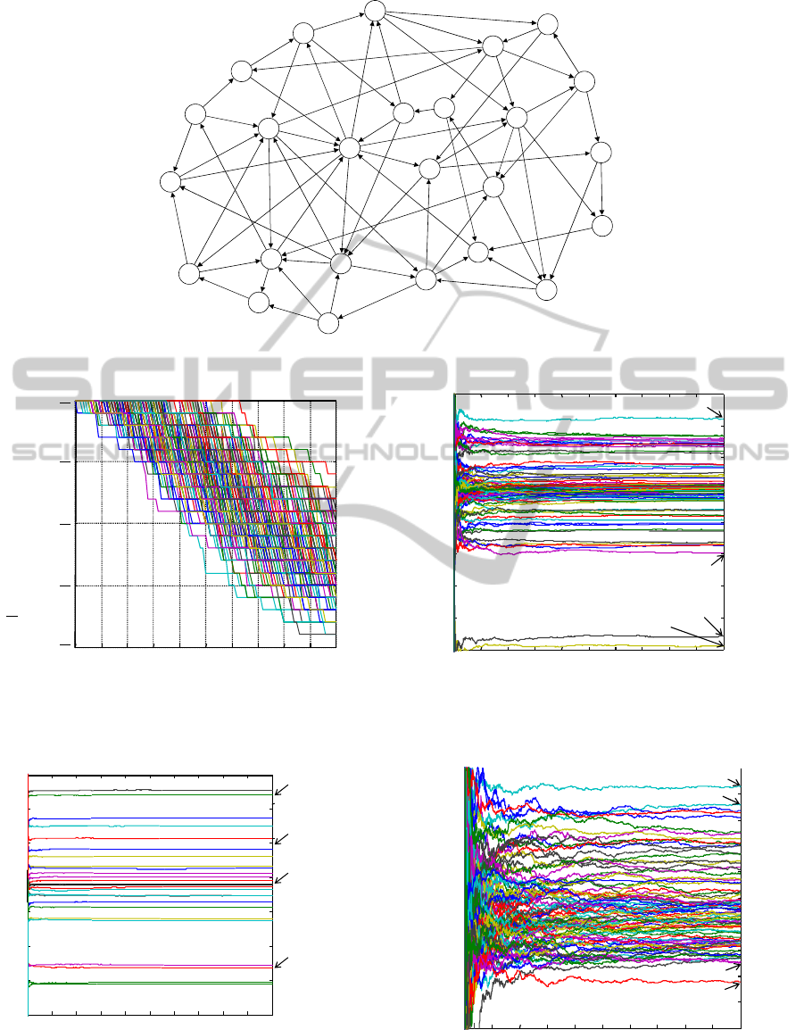
Figure 1: Financial flow-of-funds network with 25 companies.
Figure 2: Over-drawn time series of the average existence
probability by Monte-Carlo simulation.
Figure 3: Estimated value of existence probabilities vs
number of simulations.
Figure 4: Estimated value of ∂
∂μ
vs number of
simulations.
Figure 5: Estimated value of ∂
∂μ
⁄
vs number of simu-
lations.
1
2
3
4
5
6
7
8
9
10
11
12
13
14
15
16
17
18
19
20
21
22
23
24
25
[1]
[-1]
[1]
[-1]
[-2]
[1]
[-1]
[2]
[1]
[2]
[-1]
[1]
[-3]
[1]
[-1]
0102030405060708090100
t
5
25
10
25
15
25
20
25
25
25
Average existence probability
1
25
S
i
t
25
i1
Time
0 0.2 0.4 0.6 0.8 1.0 1.2 1.4 1.6 1.8 2.0
0.1
0.2
0.3
0.4
0.5
0.6
0.7
0.8
Number of simulations
×10
6
1
0.6719
i
0.4769
2
0.7415
3
0.2376
Estimated value of existence probabilities
-1
-0.8
-0.6
-0.4
-0.2
0
0.2
0.4
0.6
0 0.2 0.4 0.6 0.8 1.0 1.2 1.4 1.6 1.8 2.0
×10
6
∂
1
∂μ
ij
⁄
∂
1
∂μ
1,3
0.9747
⁄
∂
1
∂μ
1,20
0.9134
⁄
∂
1
∂μ
3
,
21
0.4447
⁄
∂
1
∂μ
18
,
19
0.3927
⁄
Number of simulations
Estimated value of
-0.1
-0.08
-0.06
-0.04
-0.02
0
0.02
0.04
0.06
0.08
0.1
0 0.2 0.4 0.6 0.8 1.0 1.2 1.4 1.6 1.8 2.0
Estimated value of
∂
i
∂μ
3,12
0.04944
∂
i
∂μ
10,23
0.06462
∂
i
∂μ
23,3
0.08596
∂
i
∂μ
0,7
0.07176
∂
i
∂μ
i
j
×10
6
Number of simulations
SIMULTECH2014-4thInternationalConferenceonSimulationandModelingMethodologies,Technologiesand
Applications
318

Table 1: the estimated values of
and
and their sensitivities ∂
∂μ
and ∂
∂μ
⁄
.
From Table 1, for example, edge 233 (the edge
from company 23 to company 3) turned out to have
the largest sensitivity of 0.08596 to
. Edge 07
(the flow of funds from the outside of the network to
company 7) and edge 010 (from the outside to
company 10) also had large sensitivities to
. It is
interesting that edge 233, which is an inner flow
of the network, had larger sensitivity to the average
existence probability
than did the inward flows
from the outside of the network, which increased the
total assets within the network. This would be ex-
plained by the fact that company 23 has four inward
edges, while it has only one outward edge 233. An
increasing flow of funds for 233, which clearly
had an adverse effect on the survival of company 23,
might be desirable for the survival of the many other
companies in the network.
We turn attention to the existence probability
of company 1. The top three edges having a large
effect on
were edge 13, edge 120, and edge
321 in descending order of the (absolute value of)
sensitivities. We are convinced that edge 13 and
edge 120, which are directly outward from node 1,
had large and negative sensitivities to
. It is inter-
i
1
2
3
4
5
6
7
8
9
10
11
12
13
14
15
16
17
18
19
20
21
22
23
24
25
#1 #2 #3 #4 #5 #6 #7 #8 #9 #10
23
→
30
→
70
→
10 0
→
18 10
→
23 0
→
17 0
→
20 0
→
23
→
12 3
→
24
0.08596 0.07176 0.06742 0.06573 -0.06462 0.06146 0.05095 0.04989 -0.04944 -0.04906
1
→
31
→
20 3
→
21 18
→
19 17
→
63
→
11 17
→
718
→
418
→
117
→
12
-0.9747 -0.9134 0.4447 -0.3927 -0.3461 0.3424 -0.3414 -0.3368 0.3345 -0.3238
2
→
32
→
52
→
21 0
→
23
→
20 20
→
21 6
→
220
→
26
→
23 20
→
4
-0.8100 -0.7856 -0.7707 0.6345 0.4148 -0.3370 0.3240 0.3066 -0.2995 -0.2838
3
→
21 3
→
11 3
→
20 3
→
12 3
→
24 20
→
43
→
52
→
21 1
→
20 20
→
2
-0.5485 -0.5407 -0.5334 -0.4134 -0.3956 0.3719 -0.3607 -0.2965 -0.2859 0.2798
4
→
10 4
→
94
→
17 4
→
04
→
39
→
18 24
→
95
→
95
→
10 19
→
4
-0.7510 -0.7464 -0.7339 -0.6120 -0.4982 0.4884 -0.4323 -0.3803 -0.3614 0.3497
5
→
19 5
→
45
→
95
→
10 4
→
319
→
39
→
33
→
24 3
→
12 3
→
21
-0.7143 -0.7053 -0.6733 -0.6124 0.4746 0.4496 0.4455 -0.4150 -0.3834 -0.3569
6
→
23 6
→
216
→
13 23
→
317
→
12 16
→
917
→
123
→
00
→
17 12
→
16
-1.0721 -1.0054 -0.4793 0.4554 -0.4080 -0.4065 -0.4058 0.3542 0.3474 0.3396
7
→
16 7
→
15 7
→
22 0
→
722
→
17 12
→
16 17
→
117
→
616
→
90
→
17
-1.0488 -1.0205 -0.9594 0.7789 0.5961 -0.4402 -0.4348 -0.3906 0.3893 0.3809
8
→
23 8
→
023
→
315
→
13 12
→
13 23
→
012
→
16 15
→
83
→
512
→
8
-1.0896 -0.8440 0.6284 -0.5632 -0.5147 0.4214 -0.4110 0.3514 -0.2901 0.2867
9
→
25 9
→
18 9
→
025
→
24 9
→
314
→
25 18
→
424
→
19 14
→
95
→
19
-0.5920 -0.5796 -0.4650 0.3994 -0.3581 -0.3199 0.3104 -0.2640 0.2539 -0.2515
10
→
23 10
→
16 10
→
11 10
→
14 0
→
10 11
→
513
→
23 16
→
13 14
→
55
→
9
-0.8638 -0.8049 -0.7756 -0.7606 0.6648 0.4750 -0.4707 0.4213 0.4069 -0.3430
11
→
15 11
→
12 11
→
55
→
10 12
→
13 22
→
17 3
→
12 15
→
13 10
→
14 3
→
11
-0.9037 -0.8759 -0.8294 0.4712 0.4209 -0.3898 -0.3650 0.3629 -0.3574 0.3462
12
→
712
→
16 12
→
812
→
13 7
→
22 17
→
716
→
90
→
78
→
23 3
→
5
-0.6790 -0.5719 -0.5492 -0.5186 0.3617 -0.3588 0.2915 -0.2793 0.2644 -0.2593
13
→
10 13
→
23 13
→
010
→
16 10
→
11 12
→
823
→
315
→
816
→
63
→
5
-0.8373 -0.8043 -0.6842 0.5073 0.4574 -0.4472 0.4331 -0.4145 -0.3261 -0.3106
14
→
914
→
514
→
25 0
→
14 5
→
10 10
→
16 10
→
11 10
→
23 0
→
10 9
→
18
-0.8365 -0.7869 -0.7464 0.6162 0.3702 -0.3328 -0.3267 -0.3026 0.2715 0.2418
15
→
815
→
13 12
→
711
→
12 7
→
16 13
→
10 8
→
23 13
→
23 0
→
77
→
22
-1.1379 -1.1117 0.5564 -0.5426 -0.5284 0.4491 0.4376 0.4156 0.4036 -0.3907
16
→
616
→
13 16
→
913
→
10 12
→
13 10
→
14 9
→
310
→
11 9
→
18 0
→
10
-0.8364 -0.8072 -0.8043 0.5246 -0.4697 -0.4008 0.3846 -0.3574 0.3417 0.3259
17
→
12 17
→
617
→
117
→
70
→
17 21
→
12 12
→
822
→
17 12
→
13 7
→
22
-0.9313 -0.8432 -0.8264 -0.7960 0.6776 -0.5995 0.3746 0.3744 0.3742 0.3387
18
→
19 18
→
418
→
10
→
18 4
→
99
→
25 9
→
05
→
924
→
99
→
3
-0.9755 -0.9174 -0.9007 0.7450 0.5324 -0.4179 -0.3943 0.3700 0.3544 -0.3315
19
→
419
→
019
→
318
→
424
→
45
→
418
→
19 24
→
19 4
→
17 5
→
19
-1.1736 -0.8793 -0.7153 -0.6266 -0.6078 -0.5807 0.4290 0.4074 0.4007 0.3902
20
→
21 20
→
220
→
40
→
20 21
→
17 3
→
21 2
→
34
→
34
→
17 1
→
20
-0.9482 -0.9310 -0.8908 0.7290 0.4338 -0.4250 0.3988 0.3926 0.3468 0.3327
21
→
17 21
→
22 21
→
12 3
→
12 17
→
12
→
21 17
→
612
→
16 20
→
412
→
13
-0.9103 -0.8803 -0.8600 -0.4702 0.4002 0.3791 0.3728 0.3541 -0.3444 0.3119
22
→
11 22
→
17 17
→
721
→
17 7
→
16 7
→
15 11
→
12 0
→
717
→
12 11
→
5
-1.0411 -0.9813 0.6397 -0.5667 -0.5137 -0.4763 0.4563 0.4280 0.3974 0.3369
23
→
023
→
33
→
12 6
→
213
→
010
→
14 8
→
06
→
23 0
→
10 10
→
23
-0.5486 -0.4449 0.2889 -0.2859 -0.2788 -0.2577 -0.2489 0.2269 0.2241 0.2192
24
→
19 24
→
40
→
24 24
→
919
→
34
→
33
→
53
→
20 3
→
11 3
→
21
-0.8424 -0.7966 0.6685 -0.6268 0.5091 0.5016 -0.4815 -0.4246 -0.4240 -0.4064
25
→
24 25
→
024
→
99
→
39
→
18 9
→
024
→
40
→
14 4
→
314
→
25
-0.9278 -0.7619 0.5972 -0.5229 -0.4131 -0.3888 0.3871 0.3564 -0.3078 0.2978
0.1888
0.6154
0.3755
0.5610
0.4799
0.5839
0.4926
0.6510
0.5141
0.7548
0.5260
0.4141
0.4483
0.2472
0.3799
0.4284
0.1940
0.4711
0.5024
0.5322
0.4482
0.7415
0.2376
0.4635
0.4769
0.6719
Existence
Probability
The estimated sensitivities with respect to each edge
μ
ij
SensitivityEstimationbyMonte-CarloSimulationUsingLikelihoodRatioMethodwithFixed-Sample-PathPrinciple
319

esting that edge 321, which does not link to com-
pany 1 directly, had the third largest sensitivity. This
would be explained if we note that edge 321 had
the largest (and negative) effect on the survival of
company 3 and edge 13 the largest (and negative)
effect on the survival of company 1.
As seen above, we can estimate the sensitivity of
and
with respect to all 86 numbers of μ
by
Monte-Carlo simulation by using the LRM method
with the score functions derived by using the fixed-
sample-path principle. Although this example net-
work is pretty small, the LRM method with fixed-
sample-path principle can be applicable and practi-
cal for much more complicated systems with numer-
ous parameters, such as for systematic risk analysis
of complicated financial networks, traffic flow on a
complicated roadway network, and emerging “big-
data” analysis.
5 CONCLUSION
In this study, a fixed-sample-path method was pro-
posed, which derives the score function of LRM not
via the pdf fx,. The key idea is to consider the
fixed-sample-path derivative of the random variables
with respect to the parameter z
under the condi-
tion of fixing the sample path x. The boundary re-
sidual R
, which represents the correction associated
with the change of the distribution range of the ran-
dom variables in LRM, was also derived. Some
examples including the estimation of risk measures
(Greeks) of option and financial flow-of-funds net-
works showed the effectiveness of the fixed-sample-
path method.
REFERENCES
Bettonvil, B., 1989. ‘A formal description of discrete
event dynamic systems including infinitesimal pertur-
bation analysis’, European Journal of Operational Re-
search, vol. 42, no. 2, pp. 213-222.
Broadie, M., Glasserman P., 1996. ‘Estimating security
price derivatives using simulation’, Management Sci-
ence, vol. 42, no. 2, pp. 269-285.
Ho, YC., Cao XR., 1991. Simulation and the Monte Carlo
Method, Springer, 1991 edition.
Glasserman, P., 2003. Monte Carlo Methods in Financial
Engineering (Stochastic Modelling and Applied Prob-
ability), Springer, 2003 edition.
Glynn, PW., 1987. ‘Likelihood ratio gradient estimation:
an overview’, Proceedings of the 19th Winter Simula-
tion Conference, pp. 366-374.
Glynn, PW., 1989. ‘Optimization of stochastic systems via
simulation’, Proceedings of the 21th Winter Simula-
tion Conference, pp. 90-105.
Rubinstein, RY., Kroese, DP., 2007. Simulation and the
Monte Carlo Method, Wiley-Interscience, 2
nd
edition.
SIMULTECH2014-4thInternationalConferenceonSimulationandModelingMethodologies,Technologiesand
Applications
320
