
Minimizing Environmental Footprints of Data Centers under Budget and
Service Requirement Constraints
Waqaas Munawar
1
, Jian-Jia Chen
1
and Minming Li
2
1
Karlsruhe Institute of Technology, Karlsruhe, Germany
2
City University of Hong Kong, Kowloon, Hong Kong
Keywords:
Green Energy Maximization, Distributed Data Centers, Response Time, Service Level Agreement.
Abstract:
The energy consumption of data centers (DCs) has been increasing, which will continue due to the increase of
Internet traffic and stringent service level agreements (SLAs). Analogously, the protection of global and local
environments has also driven the regulation authorities to encourage energy consumers, especially corporate
entities, for the usage of green energy sources. However, the green energy is usually more expensive (up
to four to five times for some cases) than the traditional energy generated from coal and petroleum. One
essential problem for managing DCs, according to the greenness tendency, is to minimize the environmental
penalty (or equivalently to maximize the greenness) by dispatching the requests to proper DCs under the
SLA and budget constraints. This paper presents optimization techniques for dynamic workload balancing
for cloud-scale data center (DC) management. We present a model for commonly found electricity tariffs
for green energy and provide an efficient heuristic algorithm to maximize its usage while incorporating its
intermittent availability. We evaluate the presented solution with real-life traces of electricity prices and DC
workloads. Extensive evaluations support our solution’s potential to minimize the environmental penalty for
Internet service providers under the budget while fulfilling their SLAs.
1 INTRODUCTION
The awareness towards the reduction of the emission
of green house gases (GHG) is increasing for the pro-
tection of global and local environments. At present,
the information technology (IT) sector consumes sig-
nificant amount of energy. Specifically, according to a
2008 estimation, about 2% of world’s GHG emissions
come from this sector (Webb et al., 2008).
One way to control the GHG emissions is to
use the greener form of energy obtained through re-
newable sources like wind and sun instead of coal,
petroleum and nuclear. The de facto standards for
such legislation have emerged to be cap-and-trade
schemes. The essence of cap-and-trade schemes is
that a regional ‘cap’ is set on the total amount of
GHG emissions for all the businesses operating in
the region. Within the cap, the businesses trade al-
lowances (i.e. carbon credits) as needed. An example
is Europe-wide EU-ETS (Commission, 2013) which
is already in its third phase. Importantly, in cap-and-
trade the brown energy cap is reduced over time so
that total emissions are progressively reduced with an
ultimate goal of having zero emissions (Commission,
2013). This approach is being followed by indus-
try (Google, 2011). To this end, a logical optimization
goal is to maximize the usage of green energy, within
bugetry constraints - the focus of this paper.
The most common instrument for trading in cap-
and-trade schemes are Renewable Energy Credits
(RECs): each REC represents one MWh of renew-
able energy contributed to the power grid. The facili-
ties that produce this energy can be based on wind or
solar farms. Importantly, RECs are not the same as
energy. Both of these, i.e. energy and RECs, can be
sold and bought separately. When a wind or a solar
farm produces energy, it is contributed to the power
grid. Such energy can then be bought like other forms
of energy. The RECs produced in this process can
be bought separately. The term green energy is actu-
ally the sum of produced energy and RECs. Hence,
it costs more than brown energy due to the addition
of RECs (for details, see (Google, 2011)). Depend-
ing upon availabilities, the wind energy can be in the
range of 6 to 16 cents per kWh. Similarly the solar en-
ergy per kWh can range from 25 cents on sunny days
to 35 cents on cloudy days. In comparison, brown en-
ergy typically costs 3∼4 cents per kWh (SolarBuzz,
222
Munawar W., Chen J. and Li M..
Minimizing Environmental Footprints of Data Centers under Budget and Service Requirement Constraints.
DOI: 10.5220/0004934202220232
In Proceedings of the 3rd International Conference on Smart Grids and Green IT Systems (SMARTGREENS-2014), pages 222-232
ISBN: 978-989-758-025-3
Copyright
c
2014 SCITEPRESS (Science and Technology Publications, Lda.)

2013).
Data centers (DCs), being the biggest users of
electricity in the IT sector (Paul Ontellini, 2011),
have a significant environmental impact. One es-
sential problem for managing DCs, according to the
greenness tendency, is to minimize the environmental
penalty by dispatching the requests to proper DCs un-
der the service level agreements (SLAs) and budget
constraints. There have been several results in the lit-
erature, e.g., (Zhang et al., 2011), (Shah et al., 2008),
(Rao et al., 2010), (Le et al., 2010a), (Qureshi et al.,
2009). Most of these researches ((Zhang et al., 2011),
(Shah et al., 2008), (Rao et al., 2010), (Qureshi et al.,
2009)) focus on the satisfying the average response
time whereas actual SLAs often demand percentile
guarantees. In (Le et al., 2010a), the percentile guar-
antees of SLAs are considered under the setting that
the brown energy consumption is capped for each DC,
whereas, a cap per enterprise is a more realistic model
as discussed previously. In (Zhang et al., 2012), the
authors consider the effect of DCs’ demand on mar-
ket prices of electricity. Detailed discussion about the
related work follows in Section 8.
Our Contribution: This paper focuses on the
minimization of the environmental footprint of DCs
under the budget constraint and the generalized SLAs,
including percentile and average response time guar-
antees. We present a software optimization strategy
to dynamically dispatch the incoming requests from
the central hub of an Internet service provider (such
as Google or iTunes) to the distributed DCs. This
optimization problem is multifaceted by considering
many important aspects in such a setting, explained
in detail in Section 2. In our approach, we divide
the problem into subproblems to be solved individ-
ually by each DC and by the central dispatching hub.
We present a practical solution that encompasses all
the energy-consuming components in a DC. That in-
cludes the energy consumption from the infrastruc-
ture for networking, computation, and cooling de-
vices. Our solution is flexible enough to be applicable
to DCs consisting of heterogeneous servers as well
as able to accommodate different SLAs. We evaluate
this with real-world workload traces from Wikipedia
(Urdaneta et al., 2009) and varying electricity prices
from different regions in USA obtained from NYISO
(NYISO, 2013). We show that this optimization prob-
lem can be effectively and efficiently solved with our
greedy algorithm by relaxing the budget constraint
and can be easily adopted in data centers.
2 BACKGROUND
This section presents the important aspects in achiev-
ing greenness in DCs.
Varying Price of Electricity. The price of both green
and brown electricity vary temporally and geograph-
ically. Also, the variance in energy used for the re-
quests, i.e., the active energy component, is a signifi-
cant fraction of the total energy (Qureshi et al., 2009).
Hence, an appropriate service placement can result in
significant gains.
Multiple Services with Different SLAs. DCs are ex-
pected to offer more than one service to more than one
client, under different SLAs and with different pric-
ing. Majority of the previous work has focused on a
single DC providing a single service. The impact of
multiple SLAs and multiple services being offered by
a group DCs has often not been considered.
Session-based Services. In the case of session-based
services offered by DCs, not all requests can be ar-
bitrarily routed to any DC. The requests belonging to
one session must either be served by the same DC, or
context transfer be quantified.
Communication Latency due to Geographical Dis-
tance. The geographical distance between the DCs
and the front end causes additional delay in serving
the routed requests (Qureshi et al., 2009). The effect
of this delay on SLA should be considered when dis-
tributing requests.
Energy Cost of Sleep-wake Transitions. Putting a
server in a DC to sleep or bringing it back for ex-
ecuting is not free in terms of energy consumption.
Sleep-wake transitions incur additional energy costs
that need to be catered when deciding to route the in-
coming load. By selecting a server that is already in
operation, extra overhead caused by the transition can
be saved.
Energy Consumption of Infrastructure. DCs do
not only consist of servers. There are also other non-
computing devices as well like networking switches,
routers, cooling devices and lighting. The average en-
ergy consumed by these devices is almost the same
as the energy consumption of processors (typical
PUE=1.9 (Stansberry and Kudritzki, 2012)). These
devices contribute substantially toward the environ-
mental footprint of a data center and their effect must
be considered.
Energy Sources and Caps. There are three basic
sources of energy in each DC: (i) green energy har-
vested through the local resources (like a local wind
farm), (ii) green energy bought in form of carbon
credits and (iii) brown energy. Many DCs nowadays
include some local facilities to produce green energy,
e.g., (Apple Inc., 2012), (Upson, 2007). The energy
MinimizingEnvironmentalFootprintsofDataCentersunderBudgetandServiceRequirementConstraints
223
produced by the local facilities is audited and con-
verted to carbon credits (NC-RETS, 2013) which can
be used just as other credits bought at local market.
The price for these credits has to be paid in the form
of initial expenditure on the renewable energy facility.
Local wind or solar farm can produce limited supply
of green energy and its maximum production cannot
exceed its rated output. This can be considered as a
limit on availability.
3 SYSTEM MODEL
In this section we formalize the system model and dis-
cuss how we handle the the challenges discussed pre-
viously (Section 2).
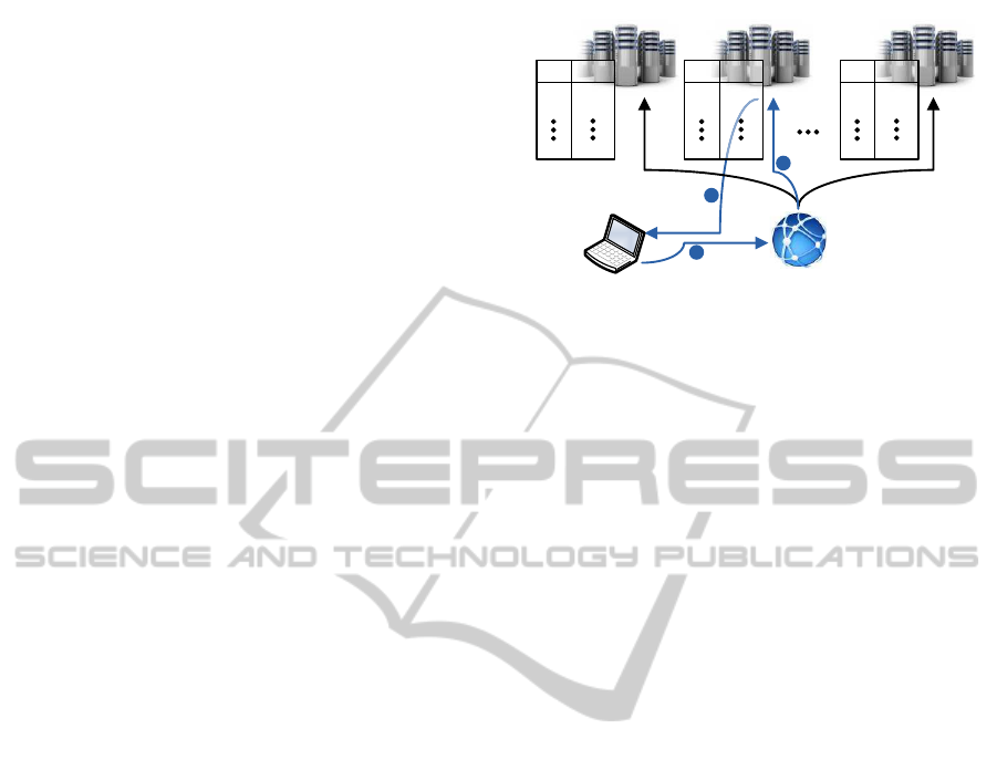
We consider a network of N DCs as shown in Fig
1. A central dispatcher receives all the requests and
dispatches them to the N DCs according to a to-be-
designed dynamic load balancing strategy. The data
centers share a common operational budget for a bud-
geting period (e.g. a month). The budgeting period
is divided into smaller control periods (e.g. an hour).
The network of data centers collaboratively provides
the total required service Λ
b
(the request rate) in a
control period b.
Energy Sources. We consider that each DC has Z
different energy sources to choose from. These can
be different forms of green or brown energy sources.
The cost to buy a unit ($ per kWh) from the j
th
energy
source in DC i during control period b is C
b,i, j
. We
assume that C
b,i, j
is time varying. Importantly, fixed-
cost energy contracts are just a special case of this
more general setting. DCs with local green energy
production facilities haveto bear the initial investment
and continuous management costs for such facilities.
These costs, amortized over time, can be considered
as the price of green energy.
When one unit of energy (kWh) is purchased from
the j
th
energy source in DC i, the associated penalty
is defined as φ
i, j
. In general, green energy sources
have none, while brown energy source has a positive
penalty.
The availability of renewable energy and carbon
credits in the market depends on the weather condi-
tions and the cap set by the legislation authorities.
Availability affects the price of energy and the cap
enforces an upper limit. We assume the j
th
energy
source in all DCs is limited to maximum usage of L
j
in the current budgeting period.
Service Level Agreements. DCs offer multiple ser-
vices to multiple clients under different SLAs. This
factor can be incorporated by dividing each DC into
smaller cells to cover all the services that should be
Front end
Data-center’s
configurations table
Data-center 1 Data-center 2 Data-center N
Reqs Energy
λ
1,1
P
1,1
λ
1,2
P
1,2
λ
1,M
P
1,M
Reqs Energy
λ
2,1
P
2,1
λ
2,2
P
2,2
λ
2,M
P
2,M
Reqs Energy
λ
N,1
P
N,1
λ
N,2
P
N,2
λ
N,M
P
N,M
Client
1
3
2
Figure 1: Arch. overview of a network of N data centers
with a typical route for a request and its reply.
provided through the DCs. Each cell is considered
as an individual DC. However, it is not that each DC
cover all the services, due to the following reasons:
(1) The overhead for maintaining the coherence of
the states is larger than the performance gains (Le
et al., 2010b). (2) Not all clients are geographically
suitably located to be served by some of the DCs be-
cause the communication latency is correlated to the
geographical distance (Qureshi et al., 2009). There-
fore the clients can be statically assigned to a subset
of DCs. Please note that SLAs that we consider are
only within the premises of service providers. Our
SLA can be combined with Internet QoS approaches
to extend the guarantees all the way to the users’ sites
(Zhao et al., 2000). For the rest of this paper, we only
present how to deal with one SLA for the simplicity of
presentation.
Session-based Services. Incoming requests from the
clients are distributed by a central dispatcher. We as-
sume that once a request has been routed, the reply
comes directly from the corresponding DC. If it is a
session-based service, all the further correspondence
is directly with the DC where the first request in the
session was assigned to. We assume that the front end
is not part of the routing process after the initial deci-
sion hence does not cause any additional latency.
DC Configuration Table. Every DC requires some
energy as an input to provide some service as output.
The required energy consumption depends upon the
service requirements as well as the hardware and in-
frastructure configurations of the DC. This behavior
can be captured in a table for energy requirement ver-
sus the maximum service (in terms of the request rate)
in a DC under the specified SLA.
We consider DCs with discretized service levels,
and each level has its required energy consumption
in a control period. Every DC has up to M different
energy usage levels (configurations) to choose from.
Each energy consumption level corresponds to a par-
ticular maximum satisfiable service requirement. A
SMARTGREENS2014-3rdInternationalConferenceonSmartGridsandGreenITSystems
224

DC i, in its k
th
configuration uses E
i,k
kWh of energy
to satisfy λ
i,k
service requirement, under the given
SLA. Once these tables have been generated for all
participating data centers, the energy requirement to
satisfy the contracted SLA for a given workload can
be simply looked up in this table.
Possible approaches for considering the energy
consumption of the servers under an SLA for a DC
can be found in the literature, e.g. the methodolo-
gies in (Guerra et al., 2008) or (Chen et al., 2011).
The energy consumed by infrastructure is also part of
the total energy consumption E
i,k
. The DC configu-
ration table forms the basis of a very general solu-
tion. It can include the energy spent on cooling, the
energy consumption of network equipment, the hard-
ware heterogeneity and various settings of SLAs. It
can potentially capture most of the relevant aspects of
a DC with selectable granularity.
Another important aspect is the energycost for the
off→on transitions of the servers in the DCs. We as-
sume that the entries in a DC configuration table al-
ready include the worst-case energy requirement for
such transitions. Hence, we do not explicitly include
them in the model. Since the transition only occurs
once (∼1 min (Le et al., 2010b)) per control period (1
hour in our model), i.e. turning the required servers on
at the beginning of every control period, adding such
worst-case energy requirements does not increase the
actual energy consumption significantly.
For notational brevity, if the available energy con-
figurations of data center i is m and m < M, we define
λ
i, j
= λ
i,m
and E
i, j
= E
i,m
for m < j ≤ M. Without
loss of generality, with respect to k, we also assume
that λ
i,k
is non-decreasing and E
i,k
is non-decreasing
as well. We assume that the first entry λ
i,1
in the data
center configuration table for DC i is 0. The corre-
sponding energy consumption E
i,1
may be 0 when the
infrastructure and the hardware does not consume any
energy when the DC is not used in the control period.
However, practically, E
i,1
> 0 and represents the en-
ergy cost of network infrastructure and other equip-
ment, e.g. lighting, etc. In essence, it is an offset that
can be added to all the entries of the configuration ta-
ble.
4 PROBLEM DEFINITION AND
FUTURE PREDICTION
4.1 Problem Statement
The objective is to minimize the total environmental
penalty in the current budgeting period while satis-
fying the service requirement with the quality of ser-
vice (QoS) as contracted in the SLA, without exceed-
ing the total budget S with the time varying energy
prices. Each DC can choose a fraction of the total
required energy in the period from any of the avail-
able sources. The optimization goal is to select an
index k
i
with 1 ≤ k
i
≤ M for DC i such that the total
environmental penalty is minimized under the service
requirement constraint
∑
N
i=1
λ
i,k
i
≥ Λ
b
∀b and the bud-
get constraint.
Summarizing this,
i, j,
=
Indices for DCs, energy sources,
k, b configurations and control periods
N = Total number of DCs
M = Max number of configurations per DC
Z = Maximum type of energy sources
B = Max control periods in budgeting period
L
j
= Maximum energy availability from j
th
source for all DCs combined (kWh)
S = total allowed cost budget for all DCs ($)
E
b,i,k
= Energy required at DC i for k
th
confguration
during b
th
control period (kWh)
φ
i, j
= penalty associated with j
th
energy source in
i
th
DC (kg of CO
2
)
C
b,i, j
= cost of j
th
energy source in i
th
DC during the
b
th
control period ($ per kWh)
Λ
b
= total service required during the b
th
control
period
λ
i,k
= service provided at DC i’s kth configuration
x
b,i, j
= In i
th
DC, portion of j
th
energy source to
fulfill the energy requirement during the b
th
control period
y
b,i,k
∈ {0,1} for all b,i,k. binary decision vari-
ables
With these symbols, the optimization problem can be
formulated as follows:
Minimize:
B
∑
b=1
N
∑
i=1
Z
∑
j=1
M
∑
k=1
y
b,i,k
· E
b,i,k
· x
b,i, j
· φ
i, j
(1a)
such that: 0 ≤ x
b,i, j
≤ 1, for all b,i, j (1b)
Z
∑
j=1
x
b,i, j
= 1, for all b,i (1c)
N
∑
i=1
M
∑
k=1
y
b,i,k
· λ
i,k
≥ Λ
b
, for all b (1d)
B
∑
b=1
N
∑
i=1
M
∑
k=1
y
b,i,k
· x
b,i, j
· E
b,i,k
≤ L
j
, for all j (1e)
B
∑
b=1
N
∑
i=1
Z
∑
j=1
M
∑
k=1
y
b,i,k
· E
b,i,k
· x
b,i, j
·C
b,i, j
≤ S. (1f)
These can be restated as:
1b: Usage of any energy source in a DC in any control pe-
riod can not be more than total energy requirement for
that data center in that control period.
1c: Sum of all the portions from all the energy sources
should satisfy the energy requirements of the DC.
MinimizingEnvironmentalFootprintsofDataCentersunderBudgetandServiceRequirementConstraints
225

1d: Provided service should satisfy the required service for
all control periods.
1e: Usage of any energy source cannot exceed its availabil-
ity in the market.
1f: The sum of the costs occurring at the DCs should re-
main within the overall budget.
4.2 Infeasibility due to Unknown
Future
A solution to the problem detailed in Equations (1a)-
(1f) will result in the optimal reduction in environ-
mental penalty. However, to solve this, we need Λ
b
and C
b,i, j
for all future control periods. This is, how-
ever, not possible. Electricity prices change on hourly
basis and the horizon for “certain” knowledge spans
only an hour in future. Similarly, as service requests
follow long term (monthly) and short term (hourly)
trends (see Figure 3), good enough predictions are
possible only for an hour in advance. Due to these
factors we transform the problem to maximize the
use green energy within a single control period. The
problem can be modified as follows for a control pe-
riod b, where 1 ≤ b ≤ B: (with modified set of old
symbols which belong only to a single control period)
Minimize:
N
∑
i=1
Z
∑
j=1
M
∑
k=1
y
i,k
· E
i,k
· x
i, j
· φ
i, j
, (2a)
such that: 0 ≤ x
i, j
≤ 1, for all i, j (2b)
Z
∑
j=1
x
i, j
= 1, for all i (2c)
N
∑
i=1
M
∑
k=1
y
i,k
· λ
i,k
≥ Λ, (2d)
N
∑
i=1
M
∑
k=1
y
i,k
· x
i, j
· E
i,k
≤ L
j
− L
b−1
j
, for all j (2e)
N
∑
i=1
Z
∑
j=1
M
∑
k=1
y
i,k
· E
i,k
· x
i, j
C
i, j
≤ ψ(S− S
b−1
). (2f)
here,
• ψ = function for budget distribution. It must satisfy:
ψ(∆) ≤ ∆. ψ(∆) can be as simple as
∆
B−b+1
or can be
complex to include the predictions of traffic and
pricing.
• L
δ
j
= Used-up quota of energy availablilty for j
th
type
of energy upto δ control period, where L
0
j
= 0.
• S
δ
= Budget consumed in the past for control periods
upto δ with S
0
= 0.
Henceforth, we tackle the problem of greening the
DCs as per Equations (2a)-(2f) i.e., according to the
methodology shown in Figure 2. For every control
!
"
#
$
Figure 2: Outline for modified methodology.
period, we first calculate the budget on basis of traffic
forecast. Predictions based on historical information
or other prediction models, e.g., (Verma et al., 2010),
(Box and Jenkins, 1994), can be adopted. In the sec-
ond step a load balancing strategy has to be designed
for the data centers under the calculated budget con-
straint and the Λ constraint with the specified SLA.
The requests are dispatched to different DCs as a re-
sult of the second step. The main focus of our method-
ology in this paper is the second step, i.e. load bal-
ancing. We assume that dispatching overhead is neg-
ligible.
Hardness. The problem formulated in Equations
(2a)-(2f) is N P -hard even for deriving a feasible so-
lution. This can be proved by reducing from the deci-
sion version of the knapsack problem.
Proof. We reduce from the decision version of the
knapsack problem. For an input instance of the knap-
sack problem, we are given N items and two constants
W and V, in which each item i has a weight w
i
and a
value v
i
. The objective of the knapsack problem is
to select a subset of the N items such that the total
weight of the selected items is less than or equal to W
and their value is larger than or equal to V. The knap-
sack problem is N P -complete (Johnson and Garey,
1979).
The reduction works as follows: We construct N
DCs such that each DC has only two configurations
for the performance and energy consumption. That
is, for DC i, λ
i,1
= 0, E
i,1
= 0, λ
i,2
= v
i
,E
i,2
= w
i
. The
performance requirement in current budgeting period
b, λ
F,b
is set to V, while the budget is set to W. The
cost to buy one unit from the brown energy source is
set to 1 as well.
Therefore, there exists a feasible solution for the
knapsack problem if and only if the reduced in-
stance for the studied problem has a feasible solu-
tion. Hence, we conclude that deriving a feasible so-
lution under budget and performance constraints for
the studied problem is N P -hard.
SMARTGREENS2014-3rdInternationalConferenceonSmartGridsandGreenITSystems
226

5 OUR SOLUTION
The drawback of solving the optimization problem
separately for each control period (Equations (2a)-
(2f)), is that the global optimization is not guaranteed.
I.e., the possibility to trade off expensive green energy
in one control period against cheaper green energy in
another control period might remain unutilized. We
show this by solving this problem optimally within
a control period through dynamic programming. Af-
ter that we present a simple greedy algorithm that, by
optimizing the budget distribution, produces better re-
sults in our simulations. Finally, we combine the pos-
itives of both approaches to form our final solution.
5.1 Dynamic Programming (DP)
5.1.1 Penalty Table for a DC
We first consider how to optimize for any DC i in a
control period when the local budget S
i
and the local
service requirement Γ
i
are given. According to the
definition, we know that we should choose the least
power-intensive configuration of the data center that
fulfills the service requirement, i.e., k
∗
with λ
i,k
∗
≥ Γ
i
.
Suppose that x
i, j
with 0 ≤ x
i, j
≤ min{1,
L
j
E
i,k
∗
} is
the fraction of the total energy purchased from the j
th
energy source in DC i. It is now clear that the objec-
tive for this case is to minimize E
i,k
∗
Z
∑
j=1
x
i, j
· φ
i, j
such
that
Z
∑
j=1
x
i, j
·C
i, j
· E
i,k
∗
≤ S
i
and
Z
∑
j=1
x
i, j
= 1. This can
be solved by using the linear programming solver in
general. Since, the green energy sources have zero
environmental penalty, the above linear programming
can be solved by a simple algebra calculation in O(Z)
time complexity given that energy sources are pre-
sorted for preference. We omit the details of algebra
here.
By iterating all possible values of S
i
and Γ
i
, we
can build the corresponding penalty table p(i, Γ
i
,S
i
)
to show the minimum penalty for DC i under the
above configurations. If it is not feasible to support
Γ
i
under budget S
i
, then, p(i,Γ
i
,S
i
) will be set to ∞.
We removethe infeasible and dominated entries in
the penalty p-table for DC i created above. An entry
p(i,λ, s) is dominated by another entry p(i, λ
′
,s
′
) if
s ≥ s
′
, λ ≤ λ
′
, and p(i,λ,s) > p(i,λ
′
,s
′
).
Suppose that the p-table has Q
i
entries for DC
i after the above procedure. The p-table has to be
generated in each control period because the penalty
incurred depends on the time-varying energy prices
which are not know a priori. For the k
th
entry in the
p-table for DC i with k ≤ Q
i
, we denote
• ℓ
i,k
as the service provided (request rates),
• s
i,k
as the allocated budget, and
• π
i,k
as the penalty stored in p(i, ℓ
i,k
,s
i,k
).
5.1.2 Building the Dynamic Programming Table
On the basis of the penalty tables (p-table) obtained
for each data center in previous step we can now build
a dynamic programming table to select the appropri-
ate configuration of every DC to provide the total re-
quired service.
Suppose that P(i, λ, s) is the minimum penalty for
the first i DCs under the budget s to provide the ser-
vice requirement (total request rate) λ. For brevity,
when λ < 0 or s < 0, we define P(i,λ,s) as ∞. Clearly,
for λ ≥ 0 and s ≥ 0, we know that
P(1, λ, s) = p(1, λ, s). (3)
Where p-table is from previous section.
For i = 2, 3,...,N, thefollowing recursiveformula
can be adopted to minimize the total penalty P under
budget s ≥ 0 and service requirement λ ≥ 0:
P(i,λ,s) = min
k=1,2,...,Q
i
{P(i− 1,λ− ℓ
i,k
,s− s
i,k
)
+π
i,k
}. (4)
Clearly, P(N, Λ, S) is the minimum penalty for
distributing the requests and the budgets. The stan-
dard dynamic programming technique can be adopted
and the solution can be obtained via backtracking
from P(N,Λ,S). The time complexity for calculat-
ing a single entry P(i, λ, s) based on Equation (4) is
O(Q
i
). To build the table correctly, we have to calcu-
late P(i,λ,s) from i = 1, 2, . . . , N and from λ = 0 to Λ
and from s = 0 to s = S sequentially. This gives the
overall time complexity O(NSΛQ
max
), where Q
max
is
max
i
Q
i
.
Optimality and Complexity. The above presented
DP approach derives the optimal solution to minimize
the environmental penalty for a control period. How-
ever, in the problem scale, some level of discretization
in both budget and service is mandatory. Appropriate
discretization results in a smaller global penalty table
(P) and this reduces the computation complexity. The
construction of the table P depends on how we dis-
cretize the values of λ from 0 to Λ and the values of s
from 0 to S. The complexity can be reduced by round-
ing down s
i,k
and s to the nearest integer multiple of
a given number, let’s say, I
s
. That is, s
′
i,k
is
j
si,k
I
s
k
I
s
.
Similarly, we can also round down ℓ
i,k
and λ to the
MinimizingEnvironmentalFootprintsofDataCentersunderBudgetandServiceRequirementConstraints
227

nearest integer multiple of a given number, let’s say,
I
λ
. That is, ℓ
′
i,k
is
j
ℓi,k
I
λ
k
I
λ
. Then I
s
and I
λ
can serve
as the discretization factors of budget S and Λ. This
makes the time complexity to O(N
S
I
s
Λ
I
λ
Q
max
).
5.2 Greedy Algorithm
We now present a heuristic algorithm based on a
greedy strategy without building the penalty p-table
constructed in Section 5.1.1. The two important fac-
tors to be considered are the penalty and the budget.
These two factors are inversely related, i.e. to reduce
penalty more budget has to be paid and vice versa. We
devise a heuristic strategy which strives to minimize
the weighted sum of both.
Suppose that the DC i has been decided to use the
k
th
i
configuration. That is, it will provide λ
i,k
i
service
with E
i,k
i
energy consumption. Suppose that x
i, j
with
0 ≤ x
i, j
≤ min{1,
L
j
E
i,k
i
} is the fraction of the total en-
ergy purchased from the j
th
energy source in DC i. If
k
i
is given for every DC i, the objective for this case
is to
minimize
N
∑
i=1
E
i,k
i
Z
∑
j=1
x
i, j
· φ
i, j
(5a)
such that
N
∑
i=1
Z
∑
j=1
x
i, j
· E
i,k
i
C
i, j
≤ S, (5b)
Z
∑
j=1
x
i, j
= 1, for all i (5c)
N
∑
i=1
E
i,k
i
· x
i, j
≤ L
j
. for all j (5d)
The above linear programming can be solved opti-
mally by using a linear programming solver or via
linear algebraic calculation with less time complex-
ity. We omit the details for the algebra due to the
space limitation.
The algorithm works as follows: all the DCs are
set to their lowest service setting, i.e. k
i
= 1 and we
check for feasibility of this setting in terms of budget
and service by verifying the feasibility and solving the
optimal solution for Equation (5a). If
∑
N
i=1
λ
i,k
i
is no
less than Λ, the algorithm terminates; otherwise it in-
creases one DC i
∗
among the DCs to the next config-
uration k
i
∗
+ 1. The selection of i
∗
is as follows:
Suppose that the current solution has set k
i
. By ad-
vancing only DC i to the configuration k
i
+ 1, we can
find the optimal setting in Equation (5a) for minimiz-
ing the penalty under this setting. Please note that the
penalty is set to ∞ if there is no feasible solution for
Equation (5a). By advancing the configuration of DC
i, suppose that ∆
service
i
is additional service, ∆
penalty
i
is the additional penalty, and ∆
budget
i
is the additional
Algorithm 1: The Greedy Algorithm.
Input: Data center configuration table for all DCs,
Service requirement: Λ, Budget: S, weights:
w
b
, w
e
Output: Configuration for all DCs: k
i
k
i
←− 1 for each DC i;
while true do
if
N
∑
i=1
λ
i,k
i
≥ Λ then
if Equation (5a) has a feasible solution then
return the solution k
i
for each DC i with
the purchase plan by solving
Equation (5a) optimally;
else
return the solution k
i
for each DC i but
with “over budgeting” by buying all
energy from the cheapest brown source;
for each DC i with k
i
< M do
∆
service
i
←− λ
i,k
i
+1
− λ
i,k
i
;
calculate ∆
budget
i
,∆
penalty
i
based on
Equation (5a);
let i
∗
be the minimum (
∆
penalty
i
∗
∆
service
i
∗
· w
b
+
∆
budget
i
∗
∆
service
i
∗
· w
e
);
k
i
∗
←− k
i
∗
+ 1;
budget (this is none-zero when the budget has not yet
been exhausted in the current solution).
For a DC i, we define two terms: brownness, i.e.
penalty caused per unit of provided service (
∆
penalty
i
∆
service
i
)
and economy, i.e. budget spent per unit of pro-
vided service (
∆
budget
i
∆
service
i
). The heuristic that we use is
brownness· w
b
+ economy· w
e
. Where w
b
and w
e
are
the weights that can be assigned to prefer brownness
over economy or vice versa.
Algorithm 1 presents the pseudo-code of the
above greedy algorithm. The worst-case number of
combinations that we have to check for different k
i
in
this algorithm is O(N
2
M), as in each while loop in Al-
gorithm 1 we consider up to N DCs and the number of
iterations in the while loop is at most NM. For each
combination, we have to solve Equation (5a). This
can be sped up by starting based on the current solu-
tion. However, solving Equation (5a) by using linear
programming solvers is already quite efficient. As we
are not able to guarantee the budget satisfaction, over
budgeting may be needed by borrowing from future
invocations, as presented in pseudo-code.
5.3 Greedy + DP (G+D)
The greedy algorithm, when allowed over-budgeting,
guarantees to find a feasible solution, if there exists
SMARTGREENS2014-3rdInternationalConferenceonSmartGridsandGreenITSystems
228

one. It keeps increasing the offered service progres-
sively in search of a feasible solution. In the worst
case, it configures all the DCs to run at maximum ser-
vice setting. However, in the average case, it finds a
feasible setting much earlier. Moreover, the heuris-
tic used for the greedy algorithm does not buy overly
expensive green energy, resulting in a efficient bud-
get usage. In comparison, the DP method finds the
optimal solution in terms of environmental penalty,
even if the cost to reduce the environmental penalty is
overly prohibitive.
We devise a method to combine both approaches
to accumulate the benefits of both: for a given control
period we execute the greedy algorithm to find a fea-
sible solution. We analyze the budget requirement of
this solution and set this as the maximum budget con-
straint for the DP method. Since the greedy algorithm
optimizes for the budget as well, its solutions are more
miserly in terms of budget usage. Setting this budget
as upper limit for DP results in a reduced search space
for dynamic programming approach. In this way we
achieve a solution which incorporates the budget op-
timization of the greedy algorithm with the optimal
search for minimal environmental penalty from DP
approach.
As G+D uses greedy and DP sequentially, its
worst case time complexity is O(N
3
M
S
I
s
Λ
I
λ
Q
max
), us-
ing the previously introduced symbols.
In the following sections we present our simula-
tion setup and evaluation results.
6 SIMULATION SETUP
We adopt the settings from (Zhang et al., 2011)
to evaluate the proposed solution by simulating the
Google’s setup for the location of DCs in the US. For
these locations, we obtain the electricity pricing infor-
mation from (NYISO, 2013). For our simulations, the
following factors are important.
Non-varying Factors include the hardware capabil-
ities of the DCs. These include server capabilities
and cooling infrastructure. We consider four DCs,
in which each data center is equipped with homo-
geneous servers, as detailed in Table 1. We use the
method in (Wang et al., 2012) to build the DC config-
uration table, presented in Section 3, by considering
50 servers in each data center. The resulting table has
at most 87 entries in each data center. Other method-
ologies like (Guerra et al., 2008) and (Chen et al.,
2011) can also be adopted for calculating the DC con-
figuration tables. Please note that the complexity of
the presented solutions does not directly depend on
the number of servers in DCs, but the number of en-
Figure 3: Wikipedia workload trace in Oct. and Nov. 2007.
tries in the DCs’ configuration tables. Even when the
servers in a DC increase, we can reduce the number
of entries in the DC configuration tables by changing
the management granularity.
The penalty for a green energy source is set to 0.
The penalty for a brown energy source is set to 1. This
multiplied byCO
2
kg generated per kWh gives actual
environmental penalty.
Time-varying Factors include energy prices. The
availability for both forms of energy does not vary.
The fluctuation in the production of green energy due
to environmental factors causes a shift in its price but
the overall availability contracted by the suppliers in
the form of RECs is fulfilled. Green energy has a
higher price than brown energy as explained in the in-
troduction (Section 1). In our simulation we assume
a surcharge of 1.5 cents and 18.0 cents per kWh for
wind and solar energy (SolarBuzz, 2013) respectively
in addition to the brown energy price. For price trace
of electricity, we use the data from NYISO(NYISO,
2013). Specifically, we use Day-Ahead price data for
Nov’07 for four regions previously mentioned.
The other time varying factor is the total service
requirement, Λ
b
. It is a random variable but over-
all it follows a weekly recurring pattern (see Figure
3). We use the actual workload trace from Wikipedia
(Urdaneta et al., 2009). We use Oct’07 for forecasting
and the Nov’07 for the actual workload.
7 EVALUATION
In this section we present the results of our evalua-
tions. We take a month as a budgeting period and an
hour as a control period. For the greedy algorithm
proposed in Section 5.2, we configure the heuristic
weights as w
b
= 10 and w
e
= 1 in Algorithm 1. The
presented algorithm (G+D) is evaluated for three main
criteria, i.e. budget allocation and usage, environmen-
tal penalty minimization and computation time. We
compare it with base line schemes of “All Green” and
“All Brown” as well as DP approach (Section 5.1) and
simple greedy (Section 5.2).
MinimizingEnvironmentalFootprintsofDataCentersunderBudgetandServiceRequirementConstraints
229
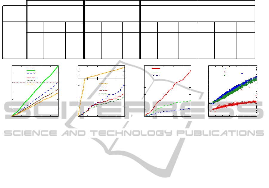
Table 1: Data center settings used for simulation (adopted from (Li et al., 2012)): Speed ratio is the ratio of the frequency by
adopting dynamic voltage frequency scaling (DVFS) to the maximum frequency in the system.
DC # 1 DC # 2 DC # 3 DC # 4
Location San Luis Valley, Colorado Los Angeles, California Oak Ridge, Tennesse Lanai, Hawaii
Processor AMD Athlon Pentium 4, 630 Pentium D950 AMD Athlon
Max freq. 3.0 GHz 3.0 GHz 3.4 GHz 3.0 GHz
Power
settings
Speed Service Power Speed Service Power Speed Service Power Speed Service Power
ratio (req/sec) (W) ratio (req/sec) (W) ratio (req/sec) (W) ratio (req/sec) (W)
1.00 750 174.09 1.00 750 93.99 1.0 850 194.00 1.00 750 174.09
0.90 675 141.28 0.80 600 62.76 0.85 725 146.19 0.90 675 141.28
0.66 500 88.88 0.50 375 37.99 0.64 550 102.13 0.66 500 88.88
0.50 375 68.13 0.40 300 34.10 0.44 375 78.82 0.50 375 68.13
0.26 200 55.29 0.30 250 32.37 0.29 250 71.20 0.26 200 55.29
!
"
#
$
!
(a) Budget usage.
!
"
#$
#%"
&
(b) Method comparison.
!
"!
#!
(c) Budget vs. penalty (G+D).
0.1
1
10
100
1000
4 6 8 10 12 14 16 18
Calculation time (sec)
Problem Size (million reqs/hr)
DP
Greedy
G+D
(d) Problem size vs. calculation
time.
Figure 4: Evaluation Results.
7.1 Budget Allocation
The hourly budget is allocated as a weighted average
of current monthly budget where the weights are cal-
culated based on predictions. We adopt a simple pre-
diction scheme that predicts the number of requests
in the current control period based on the history.
Any other prediction scheme, e.g., (You and Chan-
dra, 1999; Cortez et al., 2006) can be used for better
predictions.
The budget usage comparison is presented in Fig-
ure 4(a). The maximum allowed budget was set to
USD 80k. As expected “All Brown” uses the mini-
mum amount of budget at the cost of huge environ-
mental penalty, whereas, “All Green” approach vio-
lates maximum budget constraint (see Figure 4(b)).
The proposed solution, G+D, follows the same
budget allocation as the greedy algorithm. In compar-
ison with the optimal budget allocating scheme, “All
Brown”, it uses only one eighth more budget but pro-
duces a 15 fold reduction in environmental penalty as
shown in Figs. 4(a) and 4(b). In comparison with “All
Green”, G+D uses only half the budget.
Relaxing the budget constraint results in de-
creased environmental penalty for the presented so-
lution. The result is shown in Figure 4(c). The effect
is, however, non-linear. This is because increasing
the monthly budget beyond a certain point makes the
availability of green energy the limiting factor.
For minimizing the environmental penalty, among the
presented schemes, G+D outperforms all others that
follow the budgetry constraints as shown in Fig. 4(b).
The fundamental difference between G+D and the
DP approach is the allocation of budget. Unlike DP,
G+D tries to minimize the budget usage. This pro-
vides G+D a relaxed budget constraint progressively
at subsequent control periods, as compared to the DP
approach. DP produces the optimal results in terms of
environmental penalty within a single control period.
To this end, it sometime uses excessive budget for
gaining a marginal reduction in penalty. This makes
the budget constraint tighter in subsequent control pe-
riods, resulting in higher overall penalty for dynamic
programming.
7.2 Computation Time
For the results to be useful, the maximum compu-
tation time must remain a negligible fraction of the
length of the control period. This condition can be
fulfilled by lengthening the control period. But, this,
in turn, makes the prediction horizon longer for Λ
b
and C
b,i, j
. Irrespective of the prediction scheme, this
results in deteriorated prediction quality hence affect-
ing the solution quality.
One way to decrease computation time can be to
compute the necessary tables offline. But, due to the
time-varying factors like price and availability of en-
SMARTGREENS2014-3rdInternationalConferenceonSmartGridsandGreenITSystems
230

ergies, the offline tables will be huge and unpractical.
Online computation of solution at the beginning
of every control period is the only viable option. Fig-
ure 4(d) presents the calculation time as a function
of problem size for a single control period on a nor-
mal desktop machine (Intel i3, 6GB RAM, Linux). It
is clear that the greedy algorithm is the fastest with
majority of the computation times remaining within a
second. However, G+D may take up to a minute in a
few cases. This remains suitable for a control period
of around an hour as necessitated by the electricity
price horizon. With growing problem size, the com-
putation times increases linearly for the greedy al-
gorithm and exponentially for dynamic programming
based solutions. This was expected as DP is pseudo-
polynomial time algorithm. However, G+D, still fairs
better than DP alone. The is because of the reduced
search space due to the pruning by greedy algorithm.
8 RELATED WORK
DCs being major electricity consumers in the IT sec-
tor, have been focus of lot of research to make them
environmental friendly. This can be divided into three
main categories:
Energy Conservation: These studies aim to de-
crease the energy consumption of a DC, whereas
decreased environmental footprint is a side product.
Examples include (Chase et al., 2001), (Heo et al.,
2007), (Wang et al., 2012). Mostly these aim to opti-
mize a a single DC. For example Wang et al. (Wang
et al., 2012) present a scheme to reduce power con-
sumption while fulfilling the generalized SLAs within
a single DC. The solution we present builds on top of
these schemes as we aim for multiple DC optimiza-
tion and single DC optimization is part of that.
Electricity Cost Management: These studies are
more nearer to our approach. The key difference be-
tween this category and the previous one is that, here,
multiple and geographically distributed DCs are con-
sidered. Examples in this category include (Qureshi
et al., 2009), (Li et al., 2012), (Mathew et al., 2012),
(Luo et al., 2013). Qureshi et al. (Qureshi et al., 2009)
were the first to tackle the problem of cost minimiza-
tion by exploiting the geographic variance of energy
prices but they do not consider the carbon market dy-
namics. These are also not considered in (Li et al.,
2012) and (Luo et al., 2013).
Utilizing the Green Energy: This is a relatively
new direction with only few initial studies e.g (Zhang
et al., 2011), (Shah et al., 2008), (Rao et al., 2010).
Our approach falls in this category. (Zhang et al.,
2011) present how to maximize the use of environ-
mental friendly green energy to power the servers in
DCs, while maintaining the average response time for
incoming requests. However, since they use the queu-
ing theory to model the service provision, it can not
handle generalized SLAs, for instance, in the form of
percentile guarantees. The same argument also ap-
plies to the limitations of the researches in (Rao et al.,
2010), (Le et al., 2009), (Shah et al., 2008). More-
over, (Rao et al., 2010) and (Shah et al., 2008) do not
consider time-varying workloads, multiple services,
or market interactions. Stewart and Shen (Stewart
et al., 2009) also focus on minimizing the environ-
mental penalty by reducing the use of brown energy.
They use a model in which Internet service providers
own the renewable energy farm. In contrast, we con-
sider the more general case where the renewable en-
ergy can be locally produced or bought in form of
RECs by the commercial producers and contributed
to the grid. Le et al. (Le et al., 2010a) is more thor-
ough in their approach toward the problem. They fo-
cus on cost reduction by exploiting the distributed na-
ture of DCs for dynamic request dispatching while
maintaining SLAs. They are the first ones to con-
sider carbon interactions. Our approach has two main
differences from (Le et al., 2010a): Firstly, we aim
to maximize the green energy usage within budgetary
constraints as opposed to maximizing profits within
brown energy cap. Secondly, in our solution, we di-
vide the optimization problem to smaller parts: one
to be solved by each data center and the other for the
front end. This helps two folds (i) we can include
more factors to model energy consumption, including
the infrastructure for networking, computation, cool-
ing devices, etc., and (ii) the optimization problem
can be solved more frequently because of the reduced
complexity at the front end. The latter also results in
a shorter horizon for energy price and traffic predic-
tions.
9 CONCLUSION
The environmental footprint of DCs is becoming sig-
nificant. In this paper we formalized the problem of
minimizing the environmental footprint of ISPs (or
maximizing the green energy usage) while fulfilling
the budgetary and service constraints. We showed that
this problem is a N P -hard problem and presented a
viable greedy heuristic for optimization. The solu-
tion that we presented (1) is up to date, in that, it is
based on current legislative and economic trends. (2)
It is practical. By dividing the problem into two sub-
problems and solving them separately, it gives us the
flexibility to add different kinds of SLAs and is also
MinimizingEnvironmentalFootprintsofDataCentersunderBudgetandServiceRequirementConstraints
231

validfor heterogeneousservers in a single DC. (3) It is
wholistic in nature as it is cognizant of the energy us-
age for computation hardware, the networking hard-
ware and also the cooling infrastructure of the DC.
The novelty of our approach lies in dividing the
problem into two independent steps, that is, per DC
optimization and a central optimization scheme. This
forms the basis of general solution that can include
factors like power consumption due to cooling infras-
tructure, power consumption of networking infras-
tructure, on-site renewable energy generation systems
and multiple services with multiple SLAs.
We evaluated the presented solutions with traces
of electricity prices and typical Internet workloads.
Extensive evaluations based on real data for price,
traffic and locations demonstrate efficacy of our ap-
proach.
REFERENCES
Apple Inc. (2012). Apple facilities environmental report.
http://images.apple.com/environment/
reports/docs/Apple
Facilities Report 2012.pdf.
Box, J. and Jenkins, G. (1994). Reinsel. Time Series Analy-
sis, Forecasting and Control.
Chase, J. et al. (2001). Managing energy and server re-
sources in hosting centers. In ACM SIGOPS Operat-
ing Systems Review.
Chen, J.-J. et al. (2011). Power management schemes for
heterogeneous clusters under quality of service re-
quirements. In SAC.
Commission, E. (2013). The EU emissions trading system
(EU ETS) - policies - climate action.
Cortez, P., Rio, M., Rocha, M., and Sousa, P. (2006). In-
ternet traffic forecasting using neural networks. In
IJCNN’06. IEEE.
Google (2011). Google’s Green PPAs: What, How, and
Why - R 02. Google White Papers.
Guerra, R. et al. (2008). Attaining soft real-time constraint
and energy-efficiency in web servers. In SAC.
Heo, J., Henriksson, D., Liu, X., and Abdelzaher, T. (2007).
Integrating adaptive components: An emerging chal-
lenge in performance-adaptive systems and a server
farm case-study. In RTSS, pages 227–238. IEEE.
Johnson, D. and Garey, M. (1979). Computers and in-
tractability: A guide to the theory of np-completeness.
Freeman&Co, San Francisco.
Le, K., Bianchini, R., Martonosi, M., and Nguyen, T.
(2009). Cost-and energy-aware load distribution
across data centers. HotPower.
Le, K. et al. (2010a). Capping the brown energy consump-
tion of internet services at low cost. In Green Com-
puting Conference. IEEE.
Le, K. et al. (2010b). Managing the cost, energy consump-
tion, and carbon footprint of internet services. In ACM
SIGMETRICS.
Li, J. et al. (2012). Towards optimal electric demand man-
agement for internet data centers. IEEE Transactions
on Smart Grid.
Luo, J. et al. (2013). Data center energy cost minimiza-
tion: A spatio-temporal scheduling approach. In IN-
FOCOM.
Mathew, V. et al. (2012). Energy-aware load balancing in
content delivery networks. In INFOCOM, pages 954
–962.
NC-RETS (2013). North carolina renewable energy track-
ing system (NC-RETS). http://www.ncrets.org/.
NYISO (2013). New York Independent System Operator.
http://www.nyiso.com/.
Paul Ontellini (2011). Intel CEO speaking at Dell World.
Qureshi, A. et al. (2009). Cutting the electric bill for
internet-scale systems. In ACM SIGCOMM, pages
123–134.
Rao, L. et al. (2010). Minimizing electricity cost: Opti-
mization of distributed internet data centers in a multi-
electricity-market environment. In INFOCOM, pages
1–9. IEEE.
Shah, A. J. et al. (2008). Optimization of global data center
thermal management workload for minimal environ-
mental and economic burden. Components and Pack-
aging Technologies, IEEE Transactions on, 31(1):39–
45.
SolarBuzz (2013). Cost-Competitiveness-Solarbuzz.
http://solarbuzz.com/facts-and-figures/markets-
growth/cost-competitiveness.
Stansberry, M. and Kudritzki, J. (2012). Data center indus-
try survey. Technical report, Uptime Institute.
Stewart, C. et al. (2009). Some joules are more precious
than others: Managing renewable energy in the data-
center. In HotPower.
Upson, S. (2007). The greening of google. Spectrum, IEEE,
pages 24–28.
Urdaneta, G. et al. (2009). Wikipedia workload analysis for
decentralized hosting. Elsevier Comp. Networks.
Verma, A. et al. (2010). Brownmap: Enforcing power bud-
get in shared data centers. ACM Middleware, pages
42–63.
Wang, S. et al. (2012). Power-saving design for server farms
with response time percentile guarantees. In RTAS,
pages 273–284.
Webb, M. et al. (2008). Smart 2020: Enabling the low car-
bon economy in the information age. The Climate
Group. London.
You, C. and Chandra, K. (1999). Time series models for
internet data traffic. In LCN’99. IEEE.
Zhang, Y. et al. (2011). Greenware: Greening cloud-scale
data centers to maximize the use of renewable energy.
In Middleware.
Zhang, Y., Wang, Y., and Wang, X. (2012). Electricity bill
capping for cloud-scale data centers that impact the
power markets. In ICPP.
Zhao, W., Olshefski, D., and Schulzrinne, H. G. (2000). In-
ternet quality of service: An overview.
SMARTGREENS2014-3rdInternationalConferenceonSmartGridsandGreenITSystems
232
