A Data-driven Approach to Predict Hospital Length of Stay

A Portuguese Case Study

Nuno Caetano

, Raul M. S. Laureano

and Paulo Cortez

Instituto Universit

ario de Lisboa (ISCTE-IUL), Av. das Forc¸as Armadas, 1629-026 Lisboa, Portugal

ALGORITMI Research Centre, Department of Information Systems, University of Minho, 4800-058 Guimar

aes, Portugal

Keywords:

Medical Data Mining, Length of Stay, CRISP-DM, Regression, Random Forest.

Abstract:

Data Mining (DM) aims at the extraction of useful knowledge from raw data. In the last decades, hospitals

have collected large amounts of data through new methods of electronic data storage, thus increasing the

potential value of DM in this domain area, in what is known as medical data mining. This work focuses on

the case study of a Portuguese hospital, based on recent and large dataset that was collected from 2000 to

2013. A data-driven predictive model was obtained for the length of stay (LOS), using as inputs indicators

commonly available at the hospitalization process. Based on a regression approach, several state-of-the-art

DM models were compared. The best result was obtained by a Random Forest (RF), which presents a high

quality coefﬁcient of determination value (0.81). Moreover, a sensitivity analysis approach was used to extract

human understandable knowledge from the RF model, revealing top three inﬂuential input attributes: hospital

episode type, the physical service where the patient is hospitalized and the associated medical specialty. Such

predictive and explanatory knowledge is valuable for supporting decisions of hospital managers.

1 INTRODUCTION

In the last few decades, hospitals have been stor-

ing data regarding electronic clinical information sys-

tems. Thus, there is an increasing potential of the use

of Data Mining (DM) (Fayyad et al., 1996), to facili-

tate the creation of knowledge and support clinical de-

cision making, in what is known as medical data min-

ing (Cios and Moore, 2002; Silva et al., 2006; Silva

et al., 2008).

In this work we target the prediction of the length

of stay (LOS), deﬁned in terms of the inpatient days,

which are computed by subtracting the day of admis-

sion from the day of discharge. Extreme LOS values

are known as prolonged LOS and are responsible for a

major share in the hospitalization total days and costs.

The use of data-driven models for predicting LOS is

of value for hospital management (Azari et al., 2012;

Guzman Castillo, 2012): with an accurate estimate

of the patients LOS, the hospital can better plan the

management of available beds, leading to a more ef-

ﬁcient use of resources by providing a higher average

occupancy and less waste of hospital resources.

Given the importance of LOS prediction, a large

number of studies have approached DM techniques

in this area. Instead of predicting LOS in special-

ized medical services, as in UCI (Abelha et al., 2007;

Oliveira et al., 2010; Pena et al., 2010) or internal

medicine (Kalra et al., 2010), in this study we pre-

dict generic LOS, for all hospital services, which is

more challenging task. Also, as a case study, only

one Portuguese hospital is analyzed. Nevertheless,

a large dataset is considered (data collected from

2000 to 2013 with 26462 records from 15253 pa-

tients) when compared with some of the mentioned

works (e.g., (Pena et al., 2010) only considered 110

patients and (Oliveira et al., 2010) analyzed records

from 401 patients). In addition, the attributes that

we adopt (described in Section 2) were deﬁned by

a hospital expert’s medical panel and are commonly

available at the hospitalization process. Most of these

attributes (e.g., sex, age, episode type, medical spe-

cialty) are also adopted by the literature. For instance,

the episode type is proposed in (Guzman Castillo,

2012), while the medical specialty was used in (Azari

et al., 2012). Moreover, in contrast with several liter-

ature works, such as (Pena et al., 2010; Azari et al.,

2012; Guzman Castillo, 2012; Sheikh-Nia, 2012), we

do not perform a classiﬁcation task, which requires

deﬁning apriori which are the interesting LOS class

intervals. Instead, we adopt the more informative pure

regression approach, which predicts the actual num-

407

Caetano N., Laureano R. and Cortez P..

A Data-driven Approach to Predict Hospital Length of Stay - A Portuguese Case Study.

DOI: 10.5220/0004892204070414

In Proceedings of the 16th International Conference on Enterprise Information Systems (ICEIS-2014), pages 407-414

ISBN: 978-989-758-027-7

 2014 SCITEPRESS (Science and Technology Publications, Lda.)

ber of LOS days and not classes.

DM aims at the extraction of useful knowledge

from raw data (Fayyad et al., 1996). With the

growth of the ﬁeld of DM, several DM methodologies

were proposed to systematize the discovery of knowl-

edge from data, including the tool neutral and pop-

ular Cross-Industry Standard Process for Data Min-

ing (CRISP-DM) (Clifton and Thuraisingham, 2001),

which is adopted in this work. The methodology is

composed of six stages: business understanding, data

understanding, data preparation, modeling, evaluation

and implementation.

This study describes the adopted DM approach

under the ﬁrst ﬁve stages of CRISP-DM, given that

implementation is left for future work. At the pre-

processing stage, the data were cleaned and attributes

were selected, leading to 14 inputs and the LOS tar-

get. During the modeling stage, six regression tech-

niques were tested and compared: Average Predic-

tion (AP), Multiple Regression (MR), Decision Trees

(DT) and state-of-the-art regression methods (Hastie

et al., 2008), including an Artiﬁcial Neural Network

(ANN) ensemble, Support Vector Machines (SVM)

and Random Forests (RF). The predictive models

were compared using a cross-validation procedure

with three regression metrics, including the popular

coefﬁcient of determination. Moreover, the best pre-

dictive model (RF) was opened using a sensitivity

analysis procedure (Cortez and Embrechts, 2013) that

allows ranking the input attributes and also measuring

the average effect of a particular input in the predic-

tive response.

This paper is organized as follows. Firstly, the

adopted DM approach is detailed in terms of the

CRISP-DM methodology ﬁrst ﬁve phases (Section 2).

Then, closing conclusions are drawn (Section 3).

2 CRISP-DM METHODOLOGY

In this section, we describe the main procedures and

decisions performed when following the ﬁrst ﬁve

phases of the CRISP-DM methodology for LOS pre-

diction of a Portuguese hospital.

2.1 Business Understanding

The prediction of LOS is inserted within the wider

problem of hospital admission scheduling, where

there is a pressure to increase the availability of beds

for new patients. In this particular Hospital, most pa-

tients come from the emergency department and from

the region of Lisbon. The goal was set in terms of

predicting LOS using regression models, thus favor-

ing predictions that are closer to the target values. As

a baseline business objective (to determine if there

is success), we deﬁned a coefﬁcient of determination

with a value of 0.6, which often corresponds to a rea-

sonable regression.

In terms of software, we adopted open source

tools, using structured query language (SQL) to ex-

tract data from the hospital database and the R tool

for the data analysis (http://www.r-project-org).

In particular, we adopt the rminer package (Cortez,

2010), for applying the DM regression models (i.e.,

AP, MR, DT, ANN, SVM and RF) and sensitive anal-

ysis methods.

2.2 Data Understanding

The data was collected between October 2000 and

March 2013. During this period, a total of 26462 in-

patient episodes were stored, related with 15253 pa-

tients and associated with the distinct hospital medical

specialties.

The selection of relevant data attributes for LOS

prediction was performed by an expert medical panel.

The panel was composed with 7 physicians from

different medical specialties (e.g., internal medicine,

general surgery, gynecology). The panel presented a

total of 28 attributes that were considered related with

LOS and that were analyzed in the data preparation

phase (Table 1). The ﬁrst seven rows of Table 1 are

related with the patient’s characteristics while the re-

maining rows are related with the inpatient clinical

process. The description column of the table con-

tains in brackets the attribute type (date, nominal, or-

dinal or numeric), as found in the original hospital

database.

2.3 Data Preparation

In this phase, a substantial effort was performed us-

ing a semi-automated approach to preprocess the data.

In particular, the R tool was adopted to perform an

exploratory data analysis (e.g., histograms and box-

plots) and preprocess the original dataset. The pro-

cessing involved the operations of cleaning, discard-

ing redundant attributes, handling missing values and

attribute transformations.

During the exploratory data analysis step, a few

outliers were ﬁrst detected and then conﬁrmed by the

Physicians. The respective records were cleaned: one

LOS with 2294, an age of 207 and 29 entries related

with a virtual medical specialty, used only for test-

ing the functionalities of the hospital database. After

cleaning, the database contained 26431 records.

ICEIS2014-16thInternationalConferenceonEnterpriseInformationSystems

408

Table 1: List of attributes related with LOS prediction (attributes used by the regression models are in bold).

Name Description (attribute type)

Sex Patient gender (nominal)

Date of Birth Date of birth (date)

Age Age at the time of admission (numeric)

Country Residence country (nominal)

Residence Place of residence (nominal)

Education Educational attainment (ordinal)

Marital Status Marital status (nominal)

Initial Diagnosis Initial diagnosis description (ordinal)

Episode Type Patient type of episode (nominal)

Inpatient Service Physical inpatient service (nominal)

Medical Specialty Patient medical specialty (nominal)

Origin Episode Type Origin episode type of hospitalization (nominal)

Admission Request Date Date for hospitalization admission request (date)

Admission Date Hospital admission date (date)

Admission Year Hospital admission year (ordinal)

Admission Month Hospital admission month (ordinal)

Admission Day Hospital admission day of week (ordinal)

Admission Hour Hospital admission hour (date)

Main Procedure Main procedure description (nominal)

Main Diagnosis Main diagnosis description (ordinal)

Physician ID Identiﬁcation of the physician responsible for the internment (nominal)

Discharge Destination Patient destination after hospital discharge (nominal)

Discharge Date Hospital discharge date (date)

Discharge Hour Hospital discharge hour (date)

GDH Homogeneous group diagnosis code (numeric)

Treatment Clinic codiﬁcation for procedures, treatments and diseases (ordinal)

GCD Great diagnostic category (ordinal)

Previous Admissions Number of previous patient admissions (numeric)

Then, fourteen attributes from Table 1 were dis-

carded in the variable selection analysis step: Date

of Birth (reason: reﬂected in Age); Country (99%

patients were from Portugal); Residence (30% of

missing values, very large number of nominal lev-

els); Admission Request Date (48% of missing val-

ues, reﬂected in Admission Date); Admission Date

(reﬂected in Admission Month, Day, Hour and LOS);

admission year (not considered relevant); Physician

ID (19% of missing values and large number of 156

nominal levels); Initial Diagnosis (63% of missing

values); and attributes not known at the patient’s hos-

pital admission process (i.e., GDH, GDC, Treatment,

Discharge Destination, Date and Hour). The remain-

ing 14 attributes (bold in Table 1) were used as input

variables of the regression models (Section 2.4).

Next, missing values were replaced by using the

hotdeck method (Brown and Kros, 2003), which sub-

stitutes a missing value by the value found in the most

similar case. In particular, the rminer package uses

a 1-nearest neighbor applied over all attributes with

full values to ﬁnd the closest example (Cortez, 2010).

The following attributes were affected by this opera-

tion: Education (11771 missing values), Marital Sta-

tus (10046 values), Main Procedure (19407 values)

and Main Diagnosis (19268 values).

Finally, several attributes were transformed, to fa-

cilitate the modeling stage. To reduce skewness and

improve symmetry of the underlying variable distri-

bution, the logarithm transform y=ln(x+1) was ap-

plied to the Previous Admissions and LOS variables.

This is a popular transformation that often improves

regression results for right-skewed variables (Menard,

2002). Also, the Admission Hour variable was stan-

dardized to include only 24 levels. Moreover, the val-

ues of nominal attributes with a large number of levels

were recoded/standardized to reduce the number of

levels: Education (transformed from 14 to 6 levels),

Main Procedure (from hundreds of values to 16 lev-

els) and Main Diagnosis (from hundreds to 19 levels).

Finally, using medical knowledge, we transformed

the Age numeric attribute into 5 ordinal classes: A

- lower than 15 years; B - between 15 and 44; C -

between 45 and 64; D - between 65 and 84; and E -

AData-drivenApproachtoPredictHospitalLengthofStay-APortugueseCaseStudy

409

equal or higher than 85.

2.4 Modeling

In this phase, we tested six regression methods, as

implemented in the rminer package (Cortez, 2010):

AP, MR, DT, ANN, SVM and RF. The AP is a naive

model that consists in predicting the same average

LOS (y, as found in the training set) and is used as

baseline method for the comparison. The DT is a

branching structure that represents a set of rules, dis-

tinguishing values in a hierarchical form. The MR is

a classical statistical model deﬁned by the equation:

ˆy = β

∑

i=1

(1)

where β

,...,β

are the set of parameters to be ad-

justed, usually by applying a least squares algorithm.

ANN is based in the popular multilayer perceptron,

with one hidden layer of H hidden nodes and logistic

activation functions, while the output node uses the

linear function. Since ANN training is not optimal,

the ﬁnal solution is dependent of the choice of start-

ing weights. To solve this issue, rminer ﬁrst trains N

different networks and then uses an ensemble of these

networks such that the ﬁnal output is set in terms of

the average of the distinct N

individual predictions.

The SVM model performs a nonlinear transformation

to the input space by adopting the popular Gaussian

kernel. SVM regression is achieved under the com-

monly used ε-insensitive loss function. Under this

setup, the SVM performance is affected by three pa-

rameters: γ – Gaussian kernel parameter; ε and C –

a trade-off between ﬁtting the errors and the ﬂatness

of the mapping. Finally, RF is an ensemble of T un-

pruned DT, where each tree is based on a random fea-

ture selection with up to m features from bootstrap

training samples. The RF predictions are built by av-

eraging the outputs of T trees. RF is a substantial

modiﬁcation of bagging (ﬁt of several models to boot-

strap samples of training data) and on many problems

RF performance is similar to boosting, while being

more simpler to train and tune (Hastie et al., 2008).

The rminer package full implementation details

can be found in (Cortez, 2010). Under this package,

before ﬁtting the MR, ANN and SVM models, the

input data is ﬁrst standardized to a zero mean and

one standard deviation (Hastie et al., 2008). Except

for the hyperparameters of the most complex meth-

ods (ANN, SVM and RF), rminer adopts the default

parameters of the learning algorithms, such as: MR

and ANN – BFGS algorithm, as implemented in nnet

package; DT - CART algorithm, as implemented in

the rpart package; SVM - sequential minimal opti-

mization algorithm, as implemented in the kernlab

package; and RF - Breiman’s random forest algo-

rithm, as implemented in the randomForest package.

In this work, we set N

= 3 for the ANN ensemble.

Also, heuristics were adopted to set two of the three

SVM hyperparameters (Cortez, 2010): C = 3 (for

standardized data) and ε = 3σ

log(N)/N, where

denotes the standard deviation of the predictions

given by a 3-nearest neighbor and N is the dataset

size. For RF, we adopted the default T = 500 value.

For the most complex methods, rminer uses grid

search to select the best hyperparameter values: H

for ANN, γ for SVM and m for RF. In this paper,

the grid method searches ten values for each hyperpa-

rameter (H ∈{0,1,...,9}; γ ∈ {2

−15

−13

,...,2

}; and

m ∈ {1,2,...,10}). During the grid search, the abso-

lute error is measured over a validation set (with 33%

of the training data). The conﬁguration that corre-

sponds to the lowest valiation error is selected. Fi-

nally, the selected model is retrained with all training

data.

The method used for estimating the predictive per-

formance of a model was a 5-fold cross-validation,

which divides the data into 5 partitions of equal size.

In each 5-fold iteration, a given subset is used as test

set (to measure predictive capability) and the remain-

ing data is used for training (to ﬁt the model). To

assure statistical robustness, 20 runs of this 5-fold

procedure were applied to all methods. For demon-

stration purposes, we present here a portion of the

R/rminer code used to test the RF model:

library(rminer) # load the library

# read the data:

d=read.table("data.csv",header=T,sep=",")

# execute 20 runs of 5-fold using RF:

M=mining(LOS˜.,data=d,Runs=20,

method=c("kfold",5),

model="randomforest",

search="heuristic10")

# save the results into a file:

savemining(M,"rf.results")

2.5 Evaluation

To evaluate the predictions, three regression metrics

were selected (Witten et al., 2011): coefﬁcient of de-

termination (R2), Root Mean Squared Error (RMSE)

and Mean Absolute Error (MAE). R2 is a popular re-

gression metric that is scale independent, the higher

the better, with the ideal model presenting a value of

1.0. The lower the RMSE and MAE values, the better

the predictions. When compared with MAE, RMSE

is more sensitive to extreme errors. The Regression

Error Characteristic (REC) curve is useful to compare

ICEIS2014-16thInternationalConferenceonEnterpriseInformationSystems

410

several regression methods in a single graph (Bi and

Bennett, 2003). The REC curve plots the error tol-

erance on the x-axis versus the percentage of points

predicted within the tolerance on the y-axis.

Table 2 presents the regression predictive results,

in terms of the average of the 20 runs of the 5-fold

cross-validation evaluation scheme. From Table 2,

it is clear that the best results were obtained by the

RF model, which outperforms other DM models for

all three error metrics. A pairwise t-student statisti-

cal test, with a 95% conﬁdence level, was applied,

conﬁrming that the differences are signiﬁcant (i.e., p-

value<0.05) when comparing RF with other methods.

We emphasize that a very good R2 value was achieved

(0.813), much higher than the minimum success value

of 0.6 set in Section 2.1.

Table 2: Predictive results (average of 20 runs, as measured

over test data; best values in bold).

Metrics

Method R2 MAE RMSE

AP 0.000 0.861 1.085

MR 0.641 0.446 0.650

DT 0.622 0.415 0.667

ANN 0.736 0.340 0.558

SVM 0.745 0.296 0.547

RF 0.813

0.224

0.469

– statistically signiﬁcant under a pairwise comparison

with other methods.

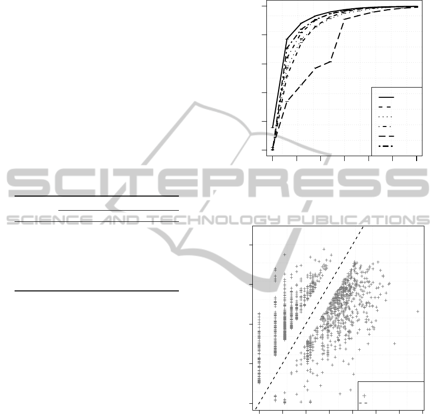
The REC analysis, shown in Figure 1, also con-

ﬁrms the RF as the best predictive model, presenting

always a higher accuracy (y-axis) for any admitted ab-

solute tolerance value (x-axis). For instance, for a tol-

erance of 0.5 (at the logarithm transform scale), the

RF correctly predicts 85.4% of the test set examples.

The quality of the predictions for the RF model can

also be seen on Figure 2, which plots the observed (x-

axis) versus de predicted values (y-axis). In the plot,

values within the 0.5 tolerance are shown with solid

circles (85.4% of the examples), values outside the

tolerance range are plotted with the + symbol and the

diagonal dashed line denotes the performance of the

ideal prediction method. It should be noted that the

observed (target) values do not cover the full space of

LOS values, as shown in Figure 2. This is an inter-

esting property of this problem domain that probably

explains the improved performance of RF when com-

pared with other methods, since ensemble methods

(such as RF) tend to be useful when the sample data

does not cover the tuple space properly. The large di-

versity of learners (i.e., T =500 unpruned trees) can

minimize this issue, since each learner can specialize

into a distinct region of the input space.

0.0 0.5 1.0 1.5 2.0 2.5 3.0

0.0 0.2 0.4 0.6 0.8 1.0

Absolute deviation

Accuracy

ANN

SVM

Figure 1: REC curves for all tested models.

0 1 2 3 4 5 6 7

0 1 2 3 4

Observed

Predicted

●

●●●

●

●●

●

●●

●

●●

●

●●

●

●●

●

●●

●

●●

●

●●

●

●●

●

●●

●

●●

●

●●

●

●●●

●

●●●

●

●●

●

●●

●

●●

●

●●

●

●●

●

●●●

●

●●

●

●●

●

●●

●

●●●

●

●●

●

●●

●

●●

●

●●

●

●●

●

●●

●

●●●

●

●●

●

●●

●

●●

●

●●●

●

●●

●

●●

●

●●●

●

●●

●

●●●●●

●

●●

●

●●

●

●●

●

●●●●●

●

●●

●

●●●

●

●●

●

●●●

●

●●

●

●●

●

●●

●

●●

●

●●

●

●●

●

●●

●

●●●●●

●

●●

●

●●

●

●●

●

●●

●

●●

●

●●

●

●●●

●

●●

●

●●

●

●●

●

●●

●

●●

●

●●

●

●●

●

●●●●

●

●●

●

●●

●

●●

●

●●

●

●●

●

●●

●

●●

●

●●

●

●●

●

●●●

●

●●

●

●●

●

●●

●

●●

●

●●

●

●●

●

●●●

●

●●

●

●●

●

●●

●

●●

●

●●●●

●

●●

●

●●

●

●●

●

●●

●

●●

●

●●

●

●●

●

●●

●

●●

●

●●

●

●●

●

●●●

●

●●●

●

●●

●

●●

●

●●

●

●●

●

●●

●

●●

●

●●

●

●●

●

●●

●

●●●

●

●●

●

●●●

●

●●

●

●●

●

●●

●

●●●

●

●●●●

●

●●

●

●●●●●

●

●●

●

●●●

●

●●

●

●●

●

●●

●

●●

●

●●

●

●●

●

●●

●

●●

●

●●

●

●●●●

●

●●

●

●●●

●

●●

●

●●●

●

●●

●

●●

●

●●

●

●●

●

●●

●

●●

●

●●

●

●●

●

●●

●

●●

●

●●

●

●●

●

●●

●

●●

●

●●

●

●●

●

●●

●

●●

●

●●

●

●●

●

●●

●

●●

●

●●

●

●●

●

●●

●

●●

●

●●

●

●●

●

●●

●

●●

●

●●

●

●●

●

●●

●

●●

●

●●

●

●●

●

●●

●

●●

●

●●

●

●●

●

●●

●

●●

●

●●

●

●●●●

●

●●

●

●●●

●

●●

●

●●

●

●●●

●

●●

●

●●

●

●●

●

●●

●

●●

●

●●

●

●●

●

●●

●

●●

●

●●

●

●●●●

●

●●

●

●●

●

●●

●

●●

●

●●

●

●●

●

●●

●

●●

●

●●

●

●●

●

●●●●

●

●●

●

●●

●

●●●

●

●●

●

●●●

●

●●

●

●●

●

●●

●

●●●

●

●●

●

●●

●

●●

●

●●●

●

●●●

●

●●

●

●●

●

●●

●

●●

●

●●

●

●●

●

●●

●

●●

●

●●

●

●●

●

●●

●

●●●

●

●●

●

●●

●

●●

●

●●

●

●●

●

●●

●

●●

●

●●

●

●●

●

●●

●

within 0.5 tolerance

other points

ideal method

Figure 2: Observed versus predicted RF values.

It should be noted that the presented predicted

results were computed over the logarithm transform

scale (see Section 2.3). In Figure 2 and within a 0.5

tolerance (solid circles), the predictions are above the

origin point (point A, x=0) and below the right upper

observed values (point B, x=4.2). This means that at

the normal scale (x

, using the inverse of the logarithm

transform), the RF model error is capable of correctly

predicting 85.4% of the examples with a real maxi-

mum error that ranges from 0.7 days (point A, x

=0)

to 26.0 days (point B, x

=65.7 days).

AData-drivenApproachtoPredictHospitalLengthofStay-APortugueseCaseStudy

411

When compared with DT and MR, the ANN,

SVM and RF data-driven models are difﬁcult to be in-

terpreted by humans. Yet, sensitivity analysis and vi-

sualization techniques can be used to open these com-

plex models (Cortez and Embrechts, 2013). The pro-

cedure works by analyzing the responses of a model

when a given input is varied though its domain. By

analyzing the sensitivity response changes, it is possi-

ble to measure input relevance (higher changes denote

a more relevant input) and average impact of an input

in the model. The former can be shown using an in-

put importance bar plot and the latter by plotting the

Variable Effect Characteristic (VEC) curve.

To extract explanatory knowledge from the RF

model and open the black-box, we applied the Data-

Based Sensitivity Analysis (DSA) method, as imple-

mented in the Importance function of the rminer

package. DSA has the advantage of being a fast

method that can measure the overall inﬂuence of a

particular input, including its iterations with other in-

puts (Cortez and Embrechts, 2013). The DSA algo-

rithm was executed over the RF model ﬁt with all

data. The obtained sensitivity responses were ﬁrst

used to rank the RF inputs, according to their rele-

vancy in the predictive model (Figure 3). Then, the

average effects of the most relevant inputs were ana-

lyzed using VEC curves (Figures 4, 5 and 6).

The input importance bar plot (Figure 3) ranks

the Episode Type (30.1% impact) as the most rele-

vant attribute, followed by Inpatient Service (12.3%)

and Medical Specialty (10.1%). Overall, the bar plot

shows a much greater inﬂuence of the inpatient clin-

ical process attributes (e.g., Episode Type, Medical

Specialty) when compared with the patients’ charac-

teristics (e.g., Education, Sex). This is an interest-

ing outcome for hospital managers. In the next para-

graphs, we detail the particular inﬂuence of the top

three inputs by analyzing their VEC curves.

Figure 4 shows the global inﬂuence of the most

relevant input (Episode Type), which is a nominal

attribute with two classes. The VEC line segments

clearly conﬁrm that the ambulatory type (scheduled

admission, typically involving a 1 day LOS) is re-

lated with an average lower LOS (0.1 in the logarithm

transform scale, 0.1 days in the normal scale) when

compared with the internment type (1.58 in the loga-

rithm scale, 3.9 days).

Next, we analyze the average inﬂuence of the In-

patient service (Figure 5). The greatest LOS is asso-

ciated with ﬁve services: medicine, average LOS of

1.45, corresponding to 3.3 days at the normal scale;

orthopedics, average of 1.39, corresponding to 3.0

days; specialties, average of 1.37, corresponding to

2.9 days; surgery, average of 1.36, corresponding to

Admission.Month

Sex

Origin.Episode.Type

Admission.Day

Age

Admission.Hour

Marital.Status

Education

Previous.Admissions

Main.Diagnosis

Main.Procedure

Medical.Specialty

Inpatient.Service

Episode.Type

0.00 0.05 0.10 0.15 0.20 0.25 0.30

Figure 3: Input importance bar plot for the RF model.

0.4 0.6 0.8 1.0 1.2 1.4 1.6

Ambulatory Internment

Figure 4: VEC line segments, showing the average inﬂu-

ence of the Episode type (x-axis) on the RF model output

(y-axis).

2.9 days; and pulmonology, average of 1.32, corre-

sponding to 2.7 days.

Finally, we analyze the third most relevant at-

tribute, the Medical Specialty (Figure 6). The inter-

nal medicine is related with the highest average LOS

(1.64, corresponding to 4.2 days). The second high-

est average LOS (1.50, corresponding to 3.5 days) is

related with orthopedics. Two Medical Specialty val-

ues are ranked third in terms of their average effect on

LOS: general surgery and urology, both related with

an average LOS of 1.40, corresponding to 3.1 days.

These results were shown to hospital specialists

and a positive feedback was obtained, conﬁrming

ICEIS2014-16thInternationalConferenceonEnterpriseInformationSystems

412

1.1 1.2 1.3 1.4

Medicine

Plastic Surgery

Surgery

Orthopedics

Pneumology

Specialties

OR Plastic Surgery

Figure 5: VEC line segments, showing the average inﬂu-

ence of the Inpatient service (x-axis) on the RF model out-

put (y-axis).

1.30 1.35 1.40 1.45 1.50 1.55 1.60 1.65

Surgery

Plastic Surgery

Internal Medicine

Ophthalmology

Orthopedics

Otorhinolaryngology

Urology

Figure 6: VEC line segments, showing the average inﬂu-

ence of the Medical specialty (x-axis) on the RF model out-

put (y-axis).

meaningful and interesting effects between these at-

tributes and the average expected LOS. Moreover,

we would like to stress that the top four relevant at-

tributes were also in agreement with several liter-

ature works. For instance, the Episode Type was

proposed by (Guzman Castillo, 2012; Freitas et al.,

2012), the Inpatient Service was adopted by (Guz-

man Castillo, 2012), the Medical Specialty was used

in (Azari et al., 2012; Sheikh-Nia, 2012), and the

Main Procedure was approached in (Abelha et al.,

2007; Guzman Castillo, 2012).

3 CONCLUSIONS

The development of the Data Mining (DM) ﬁeld has

created new exciting possibilities for the ﬁeld of med-

ical data mining. In this paper, a DM approach was

applied to estimate the length of stay (LOS) of pa-

tients at their hospital admission process. As a case

study, we analyzed recent real-world data from a Por-

tuguese hospital, involving a large dataset that in-

cluded 26462 records (from 15253 patients) and an

initial set of 28 attributes (as deﬁned by a medical

panel).

The DM approach was guided by the popular

CRISP-DM methodology, under a regression ap-

proach. After the Data Preparation phase of CRISP-

DM, a cleaned dataset (without outliers and missing

data) was achieved, with a total of 26431 records, 14

input attributes and the LOS target. During the Mod-

eling phase, six distinct regression models were com-

pared and tested, under a robust evaluation scheme

(20 runs of a 5-fold cross-validation). Finally, at

the Evaluation phase of CRISP-DM, the best results

were obtained by the Random Forest (RF) model,

which presents a very good coefﬁcient of determina-

tion value (R2=0.81, 0.21 pp higher than the mini-

mum threshold of 0.6 set in the Business Understand-

ing phase). Such model can correctly predict 85.4%

of the examples under a tolerance that ranges from 0.7

(for observed LOS of 0 days) to 26 days (for observed

LOS of 66 days). Ensemble methods methods, such

as RF, are usually usefull when the sample data does

not cover the tuple space properly and the diversity of

learners can minimize this problem

Moreover, sensitivity analysis and visualization

techniques were used to extract explanatory knowl-

edge from the best predictive model (RF). This anal-

ysis revealed a high impact of inpatient clinical pro-

cess attributes, instead of the patient’s characteristics.

In particular, the top three inﬂuential input attributes

were: the hospital episode type, the physical service

where the patient is hospitalized and the associated

medical specialty.

The obtained DM predictive and explanatory

knowledge results are valuable for hospital managers.

By having access to better estimates of what is more

likely to occur in the future and which factors affect

such estimates, hospital managers can make more in-

formed decisions (e.g., better planning of the hospital

resources), in order to accomplish their goals (e.g.,

increase the number of available beds for new admis-

sions and reduce surgical waiting lists).

In future work, we intend to explore more ensem-

ble methods, such as Adaptive Boosting (Freund and

Schapire, 1995). We will also address the Implemen-

AData-drivenApproachtoPredictHospitalLengthofStay-APortugueseCaseStudy

413

tation phase of CRISP-DM by testing the obtained

data-driven model in a real-environment (e.g., by de-

signing a friendly interface to query the RF model).

After some time, this would allow us to obtain addi-

tional feedback from the hospital managers and also

enrich the datasets by gathering more examples.

ACKNOWLEDGEMENTS

We wish to thank the physicians that participated

in this study for their valuable feedback. Also, we

would like to thank the anonymous reviewers for

their helpful suggestions. The work of P. Cortez

has been supported by FCT – Fundac¸

ao para a

encia e Tecnologia within the Project Scope: PEst-

OE/EEI/UI0319/2014.

REFERENCES

Abelha, F., Maia, P., Landeiro, N., Neves, A., and Barros,

H. (2007). Determinants of outcome in patients ad-

mitted to a surgical intensive care unit. Arquivos de

Medicina, 21(5-6):135–43.

Azari, A., Janeja, V. P., and Mohseni, A. (2012). Pre-

dicting hospital length of stay (phlos): A multi-tiered

data mining approach. In Data Mining Workshops

(ICDMW), 2012 IEEE 12th International Conference

on, pages 17–24. IEEE.

Bi, J. and Bennett, K. (2003). Regression Error Character-

istic curves. In Fawcett, T. and Mishra, N., editors,

Proceedings of 20th Int. Conf. on Machine Learning

(ICML), Washington DC, USA, AAAI Press.

Brown, M. and Kros, J. (2003). Data mining and the im-

pact of missing data. Industrial Management & Data

Systems, 103(8):611–621.

Cios, K. and Moore, G. (2002). Uniqueness of Medical

Data Mining. Artiﬁcial Intelligence in Medicine, 26(1-

2):1–24.

Clifton, C. and Thuraisingham, B. (2001). Emerging stan-

dards for data mining. Computer Standards & Inter-

faces, 23(3):187–193.

Cortez, P. (2010). Data Mining with Neural Networks and

Support Vector Machines using the R/rminer Tool. In

Perner, P., editor, Advances in Data Mining – Appli-

cations and Theoretical Aspects, 10th Industrial Con-

ference on Data Mining, pages 572–583, Berlin, Ger-

many. LNAI 6171, Springer.

Cortez, P. and Embrechts, M. J. (2013). Using sensi-

tivity analysis and visualization techniques to open

black box data mining models. Information Sciences,

225:1–17.

Fayyad, U., Piatetsky-Shapiro, G., and Smyth, P. (1996).

Advances in Knowledge Discovery and Data Mining.

MIT Press.

Freitas, A., Silva-Costa, T., Lopes, F., Garcia-Lema, I.,

Teixeira-Pinto, A., Brazdil, P., and Costa-Pereira,

A. (2012). Factors inﬂuencing hospital high length

of stay outliers. BMC Health Services Research,

12(1):265.

Freund, Y. and Schapire, R. E. (1995). A desicion-theoretic

generalization of on-line learning and an application

to boosting. In Computational learning theory, pages

23–37. Springer.

Guzman Castillo, M. (2012). Modelling patient length of

stay in public hospitals in Mexico. PhD thesis, Uni-

versity of Southampton.

Hastie, T., Tibshirani, R., and Friedman, J. (2008). The

Elements of Statistical Learning: Data Mining, Infer-

ence, and Prediction. Springer-Verlag, NY, USA, 2nd

edition.

Kalra, A. D., Fisher, R. S., and Axelrod, P. (2010). De-

creased length of stay and cumulative hospitalized

days despite increased patient admissions and read-

missions in an area of urban poverty. Journal of gen-

eral internal medicine, 25(9):930–935.

Menard, S. (2002). Applied logistic regression analysis.

Number 106. Sage.

Oliveira, A., Dias, O., Mello, M., Arajo, S., Dragosavac, D.,

Nucci, A., and Falc

ao, A. (2010). Fatores associados

maior mortalidade e tempo de internac¸

ao prolongado

em uma unidade de terapia intensiva de adultos. Re-

vista Brasileira de Terapia Intensiva, 22(3):250–256.

Pena, F., Soares, J., Peixoto, R., Jnior, H., Paiva, B.,

Moraes, F., Engel, P., Gomes, N., and Pena, G. (2010).

alise de um modelo de risco pr

e-operatrio espec-

ﬁco para cirurgia valvar e a relac¸

ao com o tempo de

internac¸

ao em unidade de terapia intensiva. Revista

Brasileira de Terapia Intensiva, 22(4):339–345.

Sheikh-Nia, S. (2012). An Investigation of Standard and

Ensemble Based Classiﬁcation Techniques for the

Prediction of Hospitalization Duration. Thesis for

Master Science Degree, University of Guelph, On-

tario, Canada.

Silva, A., Cortez, P., Santos, M. F., Gomes, L., and Neves,

J. (2006). Mortality assessment in intensive care units

via adverse events using artiﬁcial neural networks. Ar-

tiﬁcial Intelligence in Medicine, 36(3):223–234.

Silva, A., Cortez, P., Santos, M. F., Gomes, L., and Neves,

J. (2008). Rating organ failure via adverse events us-

ing data mining in the intensive care unit. Artiﬁcial

Intelligence in Medicine, 43(3):179–193.

Witten, I., Frank, E., and Hall, M. (2011). Data Mining:

Practical Machine Learning Tools and Techniques.

Morgan Kaufmann, San Franscico, USA, San Fran-

cisco, CA, 3rd edition.

ICEIS2014-16thInternationalConferenceonEnterpriseInformationSystems

414