Investigating Defect Prediction Models for Iterative Software

Development When Phase Data is Not Recorded

Lessons Learned

Anıl Aydın and Ayc¸a Tarhan

Computer Engineering, Hacettepe University, Ankara, Turkey

Keywords:

Defect Prediction, Iterative Software Development, Rayleigh Model, Linear Regression Model, Lessons

Learned.

Abstract:

One of the biggest problems that software organizations encounter is specifying the resources required and

the duration of projects. Organizations that record the number of defects and the effort spent on ﬁxing these

defects are able to correctly predict the latent defects in the product and the effort required to remove these

latent defects. The use of reliability models reported in the literature is typical to achieve this prediction, but

the number of studies that report defect prediction models for iterative software development is scarce. In this

article we present a case study which predicts the defectiveness of new releases in an iterative, civil project

where defect arrival phase data is not recorded. We investigated Linear Regression Model and Rayleigh Model

one of the statistical reliability model that contain time information, to predict the module level and project

level defectiveness of the new releases of an iterative project through the iterations. The models were created

by using 29 successive releases for the project level and 15 successive releases for the module level defect

density data. This article explains the procedures that were applied to generate the defectiveness models and

the lessons learned from the studies.

1 INTRODUCTION

As the need for software products increases day by

day, the number of software projects that address dif-

ferent types of domains also increase. A few of these

projects are developed successfully however; the ma-

jority fails (Standish, 2009). The general reason be-

hind this failure is the lack of the ability to specify and

plan resources effectively (Jones, 2004; Jones, 2006).

If the managers of software projects do not fully en-

visage the future of their projects, they can neither

plan the required resources nor identify the need for

project improvement. Thus, the completion of the

project will be delayed. This will have a negative

impact on customers and the belief in the reliability

of the project will be decreased. To overcome these

problems, organizations need to allocate resources to

estimate and predict some quality measures.

Due to the nature of software development, every

software product has defects and the employees spend

most of their time on ﬁxing the defective code seg-

ments. Estimating and predicting the defectiveness

of a software project will give organization an insight

into the future of the project; allow the redirection of

staff effort to product development and reduce delays

in the completion of project to a minimum.

In the literature, there are many studies that pro-

pose models which analyze the defectiveness of soft-

ware products and undertake defect predictions for

the future releases. The defect prediction models se-

lected or proposed by these studies generally ﬁnd so-

lutions to the speciﬁc project context (Wahyudin et

al., 2011). Finding a general model that ﬁts every

software product is hardly realistic. Every project

has speciﬁc cases, such as the domain of the soft-

ware project, the software development methodology

that is used and the experience of the staff working

on the project. These speciﬁc cases affect the defect

distribution pattern of projects thus, it was necessary

to choose an appropriate defect prediction model that

best suits our project context (Koru and Liu, 2005).

There are a number of software development

methodologies such as; Waterfall, Agile, and Iter-

ative. Each methodology proposes some develop-

ment methods or techniques. For example, the Wa-

terfall software development methodology contains

these phases; Requirements, Design, Development,

Test and Deployment which are visited in order and

Aydın A. and Tarhan A..

Investigating Defect Prediction Models for Iterative Software Development When Phase Data is Not Recorded - Lessons Learned.

DOI: 10.5220/0004888300480058

In Proceedings of the 9th International Conference on Evaluation of Novel Approaches to Software Engineering (ENASE-2014), pages 48-58

ISBN: 978-989-758-030-7

 2014 SCITEPRESS (Science and Technology Publications, Lda.)

only once. Thus, it assumes that before passing to the

next phase, all needs of the current phase have to be

fulﬁlled. For this reason, it does not give the ﬂexibil-

ity to return to solve problems that had occurred in the

previous phases. Therefore, previous phase defects

are assumed not to be contained in the latent defects.

Iterative software development, on the other hand,

consists of some iterations in the development pro-

cess to deliver the successive releases of the software

product in shorter times (Larman and Basili, 2003). In

each iteration, new requirements are identiﬁed and for

these requirements, each software development phase

will be revisited from the beginning. Thus, we can

consider each iteration as a mini waterfall (Powell and

Spanguolo, 2003). The requirements for an iteration

can be summarized as; adding a new feature to the

system, updating, changing or removing previously

developed features. Unlike Waterfall, the Iterative de-

velopment methodology gives the ﬂexibility to return

and resolve the problems that occurred at previous it-

erations.

The main goal of this study is to investigate which

prediction models best ﬁt the distributions of defect

densities at module and project level through the re-

leases of an iterative, civil project in which defect ar-

rival phase data is not recorded. Our study details the

experience and the lessons learned from this investi-

gation. As a result of the observations on defect pat-

terns of iterative projects, we decided to use a Linear

Regression Model and Rayleigh Software Reliability

Model for the module level and project level defect

densities through the iterations. For the project level,

70% of all releases

defect densities were used for

the training and constructing of the model and then,

30% of all releases

defect densities to check the ac-

curacy of the prediction model. For the module level,

three separate modules were used for the training and

constructing of prediction models and then, the de-

fect density of another module is predicted and the

accuracy of the results of the prediction is checked.

To check the accuracy and performance of each pre-

diction model, the root mean square error (RMSE),

mean absolute error (MAE) and mean magnitude rel-

ative error (MMRE) measures were used.

The framework of our study is based on a guide-

line given by (Runeson and H

ost, 2009), and the pa-

per is organized as follows: section 2 presents the

Rayleigh and Linear Regression Models; section 3

outlines related studies from the literature; section

4 gives the context of the project to be investigated

and the process defect density measure selection. Af-

ter the measure selection process, the observations on

defect density distributions and selections of suitable

models that ﬁt best to these distributions are presented

and, the analysis procedures of proposed prediction

models are given. Then, the model construction and

prediction processes are applied and the performances

of prediction models are evaluated. At the end of

this section, the threats to internal and external va-

lidity of this study are presented; section 5 shares the

lessons learned during the investigation and section 6

provides an overall conclusion.

2 BACKGROUND

Defect prediction is a process that forecasts the la-

tent defects of a project using speciﬁc techniques and

models that use historical defect distribution patterns

over a time period of the same project or another. In

addition to defect prediction, these same models and

techniques can be used to predict the defect density

and the effort required to remove the defects using

historical data. Defects in a software product follow

a speciﬁc pattern throughout the product

s life time

thus, this information helps in the prediction of the

latent defects. This process also helps managers to

envisage the future of project and estimate and plan

the resources effectively. The literature contains sev-

eral models that can predict latent defects of projects.

In this study, the Rayleigh Reliability Model and the

Simple Linear Regression Model were used to predict

an iterative civil project

s latent defect densities. A

description of the models and their functions is given

below.

2.1 Rayleigh Model

This reliability model is based on statistical distribu-

tions. It is a member of Weibull distribution fam-

ily and these types of models are generally used to

analyze the reliability of engineering products (Kan,

2002). The Rayleigh Model is usually employed to

model the distributions of the whole development life

cycle of a product. If the defect distribution pattern

follows a Rayleigh curve, we can predict the latent

defects with using the Rayleigh Model which uses

the following two functions to estimate distributions

of defects:

a) Probability Distribution Function : This

gives an estimation of the defect arrival rate at a spe-

ciﬁc time of a software product. The function is given

as;

f (t) = K ×(2t/c

) ×e

−(t/c)

(1)

b) Cumulative Distribution Function : This

gives estimation about the cumulative defect arrival

InvestigatingDefectPredictionModelsforIterativeSoftwareDevelopmentWhenPhaseDataisNotRecorded-Lessons

Learned

rate at a speciﬁc time of a software product. The func-

tion is written as follows;

F(t) = K ×(1 −e

−(t/c)

) (2)

The parameter c, located in two functions of the

Rayleigh Model, is related to the other parameter

tmax which indicates the time when the Rayleigh

curve reaches its peak. The relation between them

is;

c = t

max

√

2 (3)

K is the total defect number of software product.

F(t) shows the defect number at time t. The number

of defects found at time t

max

is equal to the 40% of

total defects (Laird, 2006). The equation proves that

claim is;

100 ×F(t

max

)/K = 100 ×(1 −e

(−0.5)

) = 40% (4)

2.2 Linear Regression Model

The regression analysis model is one of the statistical

models that indicate the relations between dependent

and independent variables (Linear regression, n.d.). It

estimates the value of the dependent variable with re-

spect to the changes in the value of the independent

variables. Regression analysis is using one or more

independent variables to create a method and esti-

mate the value of the dependent variable. If there is

only one dependent variable, then the regression anal-

ysis method is called Simple Regression. The Sim-

ple Regression Method indicates the relationship be-

tween X and Y dimensions and the relation between

them is plotted as a straight line. The Linear Regres-

sion Method is created to specify the straight line that

ﬁts most of the given set of points. This straight line

method is estimated by ﬁnding the minimum length of

a given set of points to decrease the prediction error

rate. The equation expressing the line of the Linear

Regression is;

y = a + bx (5)

In which x is the explanatory variable; y is the de-

pendent variable; b is the slope of the plotted straight

line; a is the intercept and is equal to the value where

x =0 in the given equation. The a and b values are es-

timated as follows with the given set of x and y values

(Simple linear regression, n.d.);

b =

∑

i=1

−

x)(y

−

∑

i=1

−x)

(6)

a = y −bx (7)

In this equation, the value of x is the mean of x

value set and the value of y is the mean of y value set.

3 RELATED WORKS

The defect distribution pattern differs in each project

in terms of the different project software development

lifecycles. Each lifecycle applies different techniques

and follows different steps to develop, test and main-

tain the software product. These differences affect

the defect distribution pattern. The aim in the cur-

rent study was to ﬁnd a suitable model that reﬂects

the defect distribution pattern of an iteratively devel-

oped software product. In order to do this, it is neces-

sary to understand the nature of the iterative software

development methodology. The defect arrival and re-

moval processes are the processes through a software

product

s lifecycle that help to gain an understand-

ing of that system

s characteristics (Powell and Span-

guolo, 2003). Thus, defects can be employed or in-

jected into a software system to learn how that system

behaves then; we can analyze and estimate the defect

trends in order to also predict latent defect trends.

As every project has speciﬁc cases, we need to

ﬁnd a model that ﬁts the best our projects to predict

defect distribution (Koru and Liu, 2005). The devel-

opers of every project also have speciﬁc development

styles. These individual development styles can af-

fect the defect distribution of components, modules

or projects, too. Therefore, a separate defect predic-

tion model can be built for each developer. The study

(Jiang et al., 2013) proposes to personalize each de-

fect prediction process and build prediction models

for every developer in a project.

In the literature, several models are presented that

offer a best ﬁt to defect distributions of software sys-

tems. These include; S-Shaped and Concave Shape

models. The Linear Regression Model is also among

these prediction models. One study (B

aumer et al.,

2008) compares the Linear Model with Concave and

S-Shaped models to show that the Linear Model also

gives as good performance as the other software reli-

ability growth models.

In another study (Abrahamsson et al., 2007), dy-

namic prediction models are constructed at the end

of each iteration to predict the defects of the new it-

eration. The new prediction model is created using

predictor values speciﬁc to that iteration and the pre-

vious iterations are given as an additional input. This

feature gives the prediction model a dynamic charac-

teristic. However, we choose to construct a prediction

model using historical defect data belonging to com-

pleted modules of a project to model and observe the

overall project level and module level defect trends.

Software Reliability Growth Models (SRGMs) are

also used to estimate and predict the reliability of soft-

ware products. The Rayleigh Model is one of the

ENASE2014-9thInternationalConferenceonEvaluationofNovelSoftwareApproachestoSoftwareEngineering

SRGMs that are generally used to estimate the soft-

ware project quality. This model presents equations

to estimate these reliability measures. In literature,

there are studies that use these equations to predict the

number of defects (Vladu et al., 2011), defect density,

defect removal effort and project release date (Qian et

al., 2010).

COQUALMO is another estimation model that

is presented in the literature (Hong et al., 2008;

Madachy et al., 2010) and it can be used to predict

the defect density of software products. However,

COQUALMO needs information concerning the soft-

ware product development phase and our defect data

do not contain this information. There are few predic-

tion studies in the literature that addresses this kind

of lack of data. In this study, we present a prediction

process that does not use project phase information,

which is an important contribution of this study.

The models explained in this study use the histori-

cal defect density data of an iterative software project.

As in study (B

aumer et al., 2008), we used Linear Re-

gression Model and as in studies (Vladu et al., 2011;

Qian et al., 2010), we used the Rayleigh Model to pre-

dict defect densities of latent defects. In the literature,

there are not many studies that address the defect pre-

diction process of an iterative software product. Fur-

thermore, no study was found that analyzes both the

module level and project level defect densities over it-

erations using the Linear and Rayleigh Models. This

is the main contribution of the current study to the

literature together with the sharing of our experience

and the lessons learned.

4 CASE STUDY

This section describes the current study that analyzes

the defect density distribution over iterations of an it-

erative, civil software project of a CMMI ML3 or-

ganization. Then, the constructed prediction Linear

Regression Models and Rayleigh Models of module

level and project level defect densities are explained.

4.1 Project Context

The project is an iterative, civil project and consisting

of several modules developed over 3 years. There are

several teams (containing 5 to 7 people) which are re-

sponsible for at least one of these modules. The whole

project team consists of about 30 people and turnover

of the team members has been low during the project.

Defects reported by the development team, test

team and the project customers are saved in an issue

tracker program. A reported defect is analyzed by the

relevant team leader and assigned to one of the team

members who will resolve it. The team member re-

solves the defect and then another team member, as-

signed by team leader, veriﬁes that the defect has been

resolved.

The project is developed based on subsequent re-

leases. There are main and sub releases in project.

Each main release developed over 4 to 6 weeks and

follows the methodologies identiﬁed by the iterative

software development. Thus, each main release is

considered to be iteration. Main releases consist of

sub releases that are generally developed over 5 to

7 days and released in the following order; after de-

velopment of new requirements, after testing newly

developed features and resolving the found defects

through testing activities, after deploying and resolv-

ing the defects reported by customer. Therefore, with

these activities through the sub releases, the needs of

iterative development phases are fulﬁlled.

4.2 Measure Usability Assessment

Before generating the defect density prediction mod-

els for project under investigation, we assessed the

usability of essential measures for prediction. We

chose to predict the defect density of the project and

verify that the constructed models generate good re-

sults. The defect density measure is a derived mea-

sure and generated from measures of the defect count

and number of lines of code. To evaluate the usabil-

ity of the defect density measure, we have to deter-

mine the usability of the base measure which are; the

defect count and number of lines of code. To check

the usability of these measures, we used Measure Us-

ability Questionnaire (MUQ) (Tarhan and Demir

ors,

2012). There are two kinds of MUQ for base mea-

sures and derived measures. The questionnaire con-

sists of questions to evaluate the data availability and

usability of measures. Due to the space constraint,

the questionnaire cannot be provided here. However

we should note that the information given in the com-

pleted questionnaires for the defect count, number of

lines of code, and defect density indicated that the

data for these measures fulﬁll the requirements of the

measure usability. In particular, the data availability

part of MUQ assists in the choice of suitable modules

that can be used in the current study.

4.3 Observations on the Defect

Distributions and the Speciﬁcation

of Research Questions

For the current study, to observe the defect density

distributions, we analyzed defect densities at different

InvestigatingDefectPredictionModelsforIterativeSoftwareDevelopmentWhenPhaseDataisNotRecorded-Lessons

Learned

levels of project, such as the module level and project

level. As every level of project shows a different dis-

tribution pattern, we chose a model that ﬁts best to

each level. For this, we calculated defect densities

and draw distributions over iterations.

At project level, we observed that, because of the

nature of the iterative development, newly arriving re-

quirements for each iteration cause the defect arrival

rate to be stable. In other words, the defects occurring

in any iteration generally stays at the same level. As

a consequence, if we observe the cumulative defects

over iterations, the defect distribution pattern seems

to be a straight line. Hence, we chose to apply Sim-

ple Linear Regression Model to predict the defects for

the new releases of the project. However, we also ob-

served that, the defect density data shows a decrease

in later releases. For this reason, we also analyzed the

defect density of project with the cumulative Rayleigh

distribution. In our study, the defect densities of 29 it-

erations were analyzed to predict the defect densities

at project level.

Before determining the model to be used at mod-

ule level, we analyzed the cumulative defect densi-

ties of 14 modules of the project. 10 of these 14

modules showed Rayleigh-like distribution and the

other 4 modules showed S-shaped distribution. We

did not choose an S-Shape model to predict the de-

fect densities because the 4 modules were not com-

pleted and they have few data points. In other words,

they show this S-Shaped pattern with a small num-

ber of iterations. On the other hand, the modules that

have a Rayleigh-like pattern are generally completed

or close to completion modules and have more data

points. These modules show a Rayleigh distribution

pattern because the modules are developed through

releases and when the requirements for these mod-

ules are fulﬁlled, the defect arrival rate for each mod-

ule decreases. Thus, the defect distribution of these

modules over the iterations shows a different pat-

tern from the defect distribution pattern of the over-

all project. So, for module level defect prediction, we

chose Rayleigh Model. We also analyzed the module

level defect densities with a Linear Regression Model

to compare with the results from the Rayleigh Model

prediction. The defect distributions of the three mod-

ules used in this study were analyzed through 15 it-

erations. These three modules were selected because

they have same number of data points.

After determining the models that ﬁt best the de-

fect density distributions, we constructed the predic-

tion models and tested the performance of these mod-

els. Our study was based on the following research

questions:

1: What is the performance level of the Linear Re-

gression Model in predicting the overall project de-

fectiveness in iterative software development?

2: What is the performance level of the Rayleigh

Model in predicting the overall project defectiveness

through the iterations?

3: What is the performance level of the Linear Re-

gression Model in predicting the module level defec-

tiveness in iterative software development?

4: What is the performance level of the Rayleigh

Model in predicting the module level defectiveness

through the iterations?

4.4 Analysis Procedure

To construct the defect density prediction model, it

is necessary to analyze the data and undertake various

processes. To explain these processes, we create anal-

ysis procedures as stages. The stages for each model

are given below.

In procedures, we use two parametric values. The

parametric value n, in analysis procedures, is equal

to the number of modules or projects that are used as

training data of the models. In this study, we con-

structed models for 3 modules and a project, so for

this study the value of n for modules is 3 and for the

project is 1.

The value m in the Linear Model procedure is also

parametric and this value is equal to the percentage of

all the release numbers. For our study, the value of

m is 70, which means the 70% of all releases will be

used to train and construct the Linear Model at project

level. The remainder of the defect densities of all re-

leases, that means 30% of all releases, was used to

test the performance of the constructed model.

The Rayleigh Model:

1) Gather the module or project length and defect

data

2) For each release, calculate defect density by di-

viding the number of defects recorded in that period

by module or project length

3) Depict the cumulative defect density against re-

leases as Rayleigh curves

4) Estimate the K and tmax values of the Rayleigh

Cumulative Distribution Function

5) Construct the Rayleigh Models for n number of

modules or projects that are used for training

6) Estimate the mean K and tmax values of

modules

Rayleigh Models

7) Construct the Rayleigh Prediction Model

8) Predict defect densities and estimate perfor-

mance of prediction results

The Linear Model:

ENASE2014-9thInternationalConferenceonEvaluationofNovelSoftwareApproachestoSoftwareEngineering

1) Gather the module or project length and defect

data

2) For project level, use m% of releases for the

module level, use n number of modules to calcu-

late defect density by dividing the number of defects

recorded in that period by module or project length

3) Depict the cumulative defect density against re-

leases; as data points

4) Estimate the a and b values of the Linear Re-

gression Function

5) Construct the Linear Regression Prediction

Model

6) Predict the defect densities and estimate perfor-

mance of prediction results

4.5 Model Construction

4.5.1 Module Level Model Construction

Following the stages given in the analysis procedure,

we constructed the Rayleigh Cumulative Distribution

Function Models for three separate modules labeled

and M

. The defect density distributions of

the modules show patterns like Rayleigh curve. While

constructing the models, we calculated the value of K

(total defect density) using the 40% principle (Laird,

2006). In other words, at time t

max

where the defect

density distribution reaches its peak, the found de-

fect density equals 40% of total defect density. Table

1 shows the constructed Rayleigh CDF Model func-

tions.

Table 1: Rayleigh Cumulative Distribution Functions of

modules.

Module Name Rayleigh CDF

F(t) = 18.1 ×(1 −e

−(t

/18)

)

F(t) = 13.53 ×(1 −e

−(t

/98)

)

F(t) = 9.25 ×(1 −e

−(t

/72)

)

After constructing the Rayleigh Models of defect

densities of modules M

and M

, we also used

these defect densities to construct Linear Models for

these modules. The Linear Models for the M

and M

modules are constructed and tested for 15 re-

leases or iterations. We used the Linear Regression

Model equation given in section 2.2 to ﬁnd the equa-

tion of these three modules

Linear Model through

15 releases. Table 2 shows the equations of the con-

structed Linear Models of M

and M

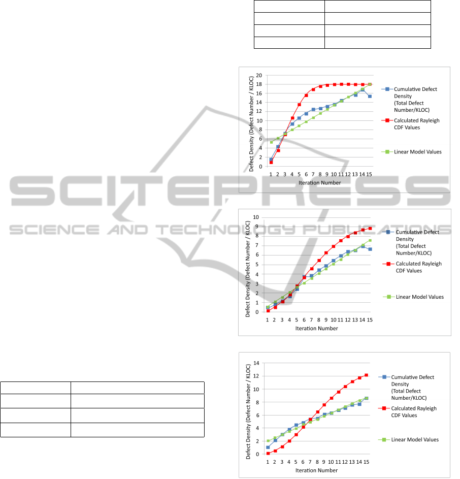
Figure 1 shows the distributions of actual and cal-

culated (Rayleigh CDF Model and Linear Model) cu-

mulative values of defect densities of each module

through iterations 1 to 15.

Table 2: Linear Regression Functions of M

mod-

ules.

Module Name Linear Model Equation

y = 4.437 + 0.899x

y = 0.057 + 0.5x

y = 1.593 + 0.474x

(a) M1 defect density distributions.

(b) M2 defect density distributions.

Figure 1: Module level defect density distributions.

4.5.2 Project Level Model Construction

After constructing the module level models, we used

project level defect densities to construct a Linear

Model and a Rayleigh Model. The Linear Model was

constructed and tested for 29 releases or iterations.

We split these releases

defect density data into train-

InvestigatingDefectPredictionModelsforIterativeSoftwareDevelopmentWhenPhaseDataisNotRecorded-Lessons

Learned

ing and testing sets. 70% of 29 releases (20 releases)

were used to construct the model and 30% of all these

releases (9 releases) were used to test these models

performances. As we calculated the K value of the

module level Rayleigh Models, we calculated the K

value of the project level Rayleigh Model using the

40% principal.

We also used the Linear Regression Model equa-

tion given in section 2.2 to ﬁnd the equation for the

Linear Model for the 20 releases. The equation of

the constructed Rayleigh Model and Linear Model is

given in Table 3.

Table 3: Project level model functions.

Model Name Model Function Equation

Rayleigh CDF F(t) = 10.04 ×(1 −e

−(t

/128)

)

Linear Model y = 0.682 + 0.319x

Figure 2 shows the distributions of the actual and

calculated (Rayleigh CDF Model and Linear Model)

cumulative values of the defect densities of project

through iterations 1 to 20.

Figure 2: Project level defect density distributions.

4.6 Prediction Results

At the module level, we create Rayleigh CDF Mod-

els and equations of M

and M

modules with

given equation in section 2.1. To create a prediction

model and an equation for module level defect den-

sities, we use the M

and M

modules

Rayleigh

CDF Models and equations, and we created another

model by calculating the mean K and t

max

values of

Rayleigh CDF function. We used this newly con-

structed Rayleigh CDF Model to estimate and predict

the defect density of another module, M

and com-

pared the predicted defect density result with actual

defect density of M

We also created a Linear Prediction Model using

the linear functions of modules M

and M

. For

this, with using the linear function constants of mod-

ules M

and M

, we calculated the mean a and b

values of linear functions given in section 2.2. Table 4

presents information about Rayleigh CDF Prediction

Model and Linear Prediction Model of module M

Table 4: Model functions of M

module.

Model Name Model Function Equation

Rayleigh CDF F(t) = 13.63 ×(1 −e

−(t

/56)

)

Linear Model y = 2.027 + 0.624x

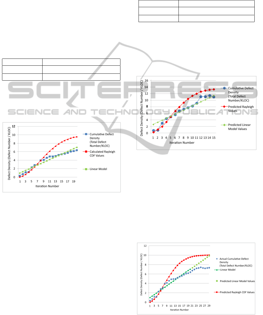
After constructing the Linear and Rayleigh Pre-

diction Models of module M

, we calculated the cu-

mulative defect densities of each iteration for mod-

ule M

using this prediction models. Figure 3 shows

the actual and predicted defect density distributions

through iterations 1-15.

Figure 3: Module level defect density prediction model dis-

tributions.

After this stage, at project level, we created a Lin-

ear Model using defect densities of 20 releases (70%

of 29 releases). We predicted the other defect densi-

ties of the 9 releases (30% of 29 releases) using the

constructed Linear Model. We also predicted the de-

fect densities of the 9 releases using the constructed

Rayleigh Model for the project level defect densities

as shown in Table 3. Figure 4 shows the additional

defect density data points of the predicted and actual

defect densities of the 9 releases.

Figure 4: Project level defect density prediction model dis-

tributions.

ENASE2014-9thInternationalConferenceonEvaluationofNovelSoftwareApproachestoSoftwareEngineering

The results show that the prediction models gen-

erally overestimate the defect densities. From this ob-

servation, it can be understood that the development

team may work effectively in developing code with

a low defect occurrence or they may remove defects

without recording them; or the testing team does not

test the projects effectively.

4.7 Prediction Performance Evaluation

Having constructed the Rayleigh and Linear Models

to predict defect densities at module level and project

level it was necessary to assess the prediction per-

formance of the models to determine how well the

models work. In literature, there are several measures

that assess the performance of prediction models. We

selected three measures to determine the goodness-

of-ﬁt; root mean square error (RMSE), mean abso-

lute error (MAE) and mean magnitude relative error

(MMRE). The RMSE measures the accuracy of the

prediction model by measuring the average magni-

tude of the error (Eumetcal, 2011). It calculates the

difference, in other word the residual, between the ac-

tual and predicted values and then, squares the differ-

ence. The square root of the residuals

mean value

gives the RMSE. The equation of RMSE is;

RMSE =

∑

i=1

−f

)

(8)

The MAE also measures the accuracy of predic-

tion model by measuring the average magnitude of the

errors (Eumetcal, 2011). The direction of errors is not

important for the MAE. The result of the MAE shows

how close the actual and predicted values are. We

expected to see little difference between the RMSE

and MAE values. This small difference between the

RMSE and the MAE means that the variation of errors

is also small. The equation of MAE is given as;

MAE =

∑

i=1

− f

| (9)

The MMRE also helps us to assess the perfor-

mance of prediction models by evaluating how much

the actual and predicted values differ relative to the

actual values. The value of MMRE ≤ 0.25 shows

that the prediction models

performances are good

(Kitchenham et al., 2001) and the models ﬁt well. The

equation of MMRE is;

MMRE =

∑

i=1

−f

(10)

Table 5 shows the RMSE, MAE and MMRE val-

ues of the module level Rayleigh and Linear Models.

Table 5: Performance values of module level prediction

models.

Rayleigh Model Linear Model

RMSE 1.777 0.969

MAE 1.515 0.664

MMRE 0.239 0.375

As shown in Table 5 the RMSE and MAE val-

ues of the Linear Model are lower than the values of

Rayleigh Model. The difference between the RMSE

and MAE values of both models are also small and

this difference shows that how much the variations

of errors are also small. However, although the Lin-

ear Model seems to have a better performance, the

MMRE value of Linear Model is greater than the ac-

ceptable result of 0.25. For this reason, it is appro-

priate to use Rayleigh Model for module level defect

density prediction.

Table 6 shows the RMSE, MAE and MMRE val-

ues of project level Rayleigh and Linear Models.

Table 6: Performance values of project level prediction

models.

Rayleigh Model Linear Model

RMSE 2.707 1.592

MAE 2.413 1.434

MMRE 0.375 0.197

As shown in Table 6, at project level, the RMSE,

MAE and MMRE values of the Linear Model are bet-

ter than Rayleigh Model. The difference between the

MAE and RMSE values of both Rayleigh and Lin-

ear Model is low which shows that the variations

of errors are small. However, at project level, the

MMRE value of the Rayleigh Model is greater than

the MMRE value of the Linear Model and this value is

also greater than the acceptable result of 0.25. For this

reason, for defect density prediction at project level,

the Linear Model is more suitable.

As we observe the results in both Table 5 and Ta-

ble 6, the performance measure values for module

level related to the RMSE and MAE values of both

Linear and Rayleigh Models are lower than the val-

ues at project level.

At module level, with respect to the RMSE and

MAE values, the Linear Model seems to have a bet-

ter performance, but the MMRE value shows that the

Rayleigh Model has more acceptable results. For this

reason, the Rayleigh Model at module level is more

usable. Modules are developed through releases and

when the requirements for these modules fulﬁlled, the

defect arrival rate for each module decreases. For this

reason, the defect density distribution of these mod-

ules over the iterations shows a Rayleigh curve like

InvestigatingDefectPredictionModelsforIterativeSoftwareDevelopmentWhenPhaseDataisNotRecorded-Lessons

Learned

pattern. To increase the performance of the Rayleigh

Model at module level, we could use defect density

data from more than three modules.

At project level, the reason why the Linear Model

is better than Rayleigh Model is that the newly arriv-

ing requirements for each iteration result in a stable

defect arrival rate and the defects occurring in any it-

eration generally remain at the same level. Thus, the

distributions of cumulative defect densities over iter-

ations converge to the Linear Model pattern.

4.8 Threats to Validity

It is important to examine the threats to the internal

and external validity of any study.

Internal validity is one of the quality test criteria

for a case study and it checks for the replicability of

the proposed analyses (Yin, 2009). It also tests the

situations that contain biases. The threats to internal

validity of this study are as follows:

- Only the defect density data of one project was

used, so we did not know whether the properties of the

projects would affect our study therefore, we could

analyze data from more projects.

- For prediction process of the module level de-

fect densities, we used three modules however; we do

not know the effect of other module properties on the

proposed model. Thus, more modules could be ana-

lyzed, possibly with other types of prediction models

to remove this threat.

- The MUQ was used to assess the usability of

measures. The questionnaire helped us to decrease

the subjectivity of this study and ensure that usable

measures and data existed before constructing statis-

tical prediction models. However, this assessment of

usability requires a particular level of expertise about

measurement, and still includes a degree of subjectiv-

ity.

- We speciﬁed the analysis procedures for both

prediction models to ensure that our study had repli-

cability. However, in order to use these procedures

at organization level it is necessary to undertake more

studies and improve our method.

Another quality test criteria is external validity

which tests the generalizability of case studies (Yin,

2009). For the current study, we cannot ensure that

these methods can be used in other contexts. There-

fore, as a future work we can analyze the defect den-

sities in relation to the properties of modules and

projects. This data can also be analyzed using other

prediction models.

5 LESSONS LEARNED

During our research, we encountered some challenges

and we feel that the lessons we learned when resolv-

ing these problems can help researchers in their work

concerning defect prediction process. First, to under-

stand the nature of development and defect removal

process of project, we spent much time considering

the defect data. We drew the defect distributions of

component level defects, release level defects, mod-

ule level defects and project level defects. We dis-

tributed these defects over the development weeks or

equally divided times such as periods of 5, 10, or

20 days. The component level and release level de-

fect distributions generally had few data points if di-

vided these defects over time into more data points,

for some of the data points there are no defects and

the actual nature of the defect distribution is lost. In

our study, the components constitute modules and the

modules constitute the project. To increase the data

points and the number of defects correspond to these

data points, we decided to use defect distributions of

the modules and the project.

We discovered that in attempting to observe the

defect distribution of development processes, how-

ever, the software development phase information

(analyze, design, development, test or maintenance)

of the defect, did not exist. This prevented us from

analyzing the defect data according to the develop-

ment phases. We cannot observe the inﬂuence of

lower life-cycle phases

quality onto the reached qual-

ity in upper-life cycle phases in software development

process. Therefore, we learned that it is necessary to

record the development phase data of that defect in

iterative development as much as in waterfall devel-

opment.

Then, we observed the defect removal effort distri-

bution over time or releases. However, while assess-

ing the measure usability of the defect removal effort,

we observed that the majority of development teams

do not enter the work log data of the defect removal

effort. For this reason, we did not use effort data

to construct a prediction model. The MUQ helped

us to determine which measure was usable in predic-

tion process. From the results of the questionnaire,

we see that a number of defects and size of product

were available, so it was decided to use defect density

(number of defects / KLOC) to construct and analyze

a prediction model. Difﬁculties were incurred when

checking the release codes and counting the lines of

module codes. Measuring the module sizes of ﬁnal re-

leases was easy but in previous releases, the code had

not been grouped by modules or components. The

classes of the components or modules in previous re-

ENASE2014-9thInternationalConferenceonEvaluationofNovelSoftwareApproachestoSoftwareEngineering

leases were located in different packages. This re-

sulted in time being spent to ﬁnd the classes of mod-

ules for the whole project. We found that the packag-

ing of classes helps any member of staff to work more

effectively. On the other hand, the project level prod-

uct size was easily achieved, because at this level, the

code size can be found by counting the lines of whole

code.

Finally, the most signiﬁcant step was deciding the

most suitable prediction model. To determine which

models that best ﬁt our situation, we used defect den-

sity distributions and we observe that the module

level defect density distribution curves converge to

the Rayleigh curves and the project level defect den-

sity distribution curve converge to a straight line that

shows a Simple Linear Regression.

6 CONCLUSIONS

In this study, we examined a defect prediction pro-

cess of an iterative, civil project in which defect ar-

rival phase data is not recorded. We analyzed the

defect density data at module level and project level

to predict the latent defect densities. By analyzing

module level distributions; we were able to analyze

defects in smaller code segments and by analyzing

the project level distributions; we analyzed the de-

fects in general. We used a software reliability growth

model (SRGM), the Rayleigh Model and the Simple

Linear Regression Model which need basic statistical

and mathematical information. To predict the defect

density of a module, we used the mean of three sep-

arate modules from the function coefﬁcients from the

Rayleigh Model and the Linear Model to create pre-

diction model functions.

The results for the project level prediction show

that the performance of the Linear Model is better

than the performance of the Rayleigh Model. From

these results, since the MMRE value of Linear Model

was under 0.25, it can be seen that the Linear Model

had a more acceptable performance. The result for the

module level shows that performance of the Linear

Model is better than the Rayleigh Model with respect

to RMSE and MAE values. However, the MMRE

value of the Linear Model does not have an accept-

able performance value (it should be less than 0.25).

The MMRE value of Rayleigh Model has a suitable

value which is smaller than the acceptable result of

0.25.

The modules used to construct a prediction model

have different complexities. So, we can increase the

performance of module level prediction results by in-

creasing the number of modules that are investigated.

At project level, due the nature of iterative develop-

ment, the defect arrival rate generally remains at the

same level and the distribution of the defect densities

converge to a Linear Model. Therefore, the Linear

Model has a higher performance than the Rayleigh

Model.

The most important lessons learned from this

study are observing the nature of defect distributions,

identifying and overcoming the lack of data, and de-

ciding the most suitable prediction model that ﬁts best

to the situation. Defect arrival and removal data col-

lection is important to model defect arrival and re-

moval patterns in relation to project phases. Due to

the nature of iterative development, a defect found

in an iteration can be ﬁxed in another iteration. It is

very important to specify in which release the defect

is found and in which release the defect is ﬁxed. An-

other important issue is the consistency and integrity

of project planning data with project defect data. De-

fect tracking tool should be capable of accessing and

working integrated with project management tool.

For future work, we are planning to include data

from more modules and projects in the models and

examine the prediction of the project schedule using

the defect removal effort spent by the project staff.

REFERENCES

Abrahamsson, P., Moser, R., Pedrycz, W., Sillitti, A., &

Succi, G. (2007, September). Effort prediction in it-

erative software development processes–incremental

versus global prediction models. In Empirical Soft-

ware Engineering and Measurement, 2007. ESEM

2007. First International Symposium on (pp. 344-

353). IEEE.

aumer, M., Seidler, P., Torkar, R., Feldt, R.,

Tomaszewski, P., & Damm, L. O. (2008). Predicting

fault inﬂow in highly iterative software development

processes: an industrial evaluation. In Supplementary

CD-ROM Proceedings of the 19th IEEE International

Symposium on Software Reliability Engineering: In-

dustry Track.

Eumetcal. (2011). Mean Absolute Error (MAE)

and Root Mean Squared Error (RMSE)

Retrieved September 23, 2013, from

http://www.eumetcal.org/resources/ukmeteocal/-

veriﬁcation/www/english/msg/ver cont var/-

uos3/uos3 ko1.htm

Hong, Y., Baik, J., Ko, I. Y., & Choi, H. J. (2008,

May). A Value-Added Predictive Defect Type Dis-

tribution Model based on Project Characteristics. In

Computer and Information Science, 2008. ICIS 08.

Seventh IEEE/ACIS International Conference on (pp.

469-474). IEEE.

Jiang, T., Tan, L., & Kim, S. (2013). Personalized defect

prediction. In Proceedings of the 28th IEEE/ACM In-

InvestigatingDefectPredictionModelsforIterativeSoftwareDevelopmentWhenPhaseDataisNotRecorded-Lessons

Learned

ternational Conference on Automated Software Engi-

neering (ASE 2013). Palo Alto, CA, November 11-15,

2013.

Jones, C. (2004). Software project management practices:

Failure versus success. CrossTalk: The Journal of De-

fense Software Engineering, 5-9.

Jones, C. (2006). Social and technical reasons for software

project failures. STSC CrossTalk June.

Kan, S. H. (2002). Metrics and Models in Software

Quality Engineering (2nd ed.). Boston, MA, USA:

Addison-Wesley Longman Publishing Co., Inc.

Kitchenham, B. A., Pickard, L. M., MacDonell, S. G., &

Shepperd, M. J. (2001, June). What accuracy statistics

really measure [software estimation]. In Software, IEE

Proceedings- (Vol. 148, No. 3, pp. 81-85). IET.

Koru, A. G., & Liu, H. (2005). Building effective defect-

prediction models in practice. Software, IEEE, 22(6),

23-29.

Laird L.(2006). In Praise of Defects Stevens Insti-

tute of Technology. Retrieved September 20, 2013,

from http://www.njspin.org/present/Linda%20Laird-

%20March%202005.pdf

Larman, C., & Basili, V. R. (2003). Iterative and in-

cremental developments. a brief history. Computer,

36(6), 47-56.

Linear regression. (n.d.). In Wikipedia.

Retrieved October 30, 2013, from

http://http://en.wikipedia.org/wiki/Linear regression

Madachy, R., Boehm, B., & Houston, D.

(2010). Modeling Software Defect Dynam-

ics. Retrieved November 1, 2013, from

http://csse.usc.edu/csse/TECHRPTS/2010/usc-

csse-2010-509/usc-csse-2010-509.pdf

Powell, J. D., & Spanguolo, J. N. (2003). Modeling defect

trends for iterative development.

Qian, L., Yao, Q., & Khoshgoftaar, T. M. (2010). Dy-

namic Two-phase Truncated Rayleigh Model for Re-

lease Date Prediction of Software. JSEA, 3(6), 603-

609.

Runeson, P., & H

ost, M. (2009). Guidelines for conduct-

ing and reporting case study research in software engi-

neering. Empirical Software Engineering, 14(2), 131-

164.

Simple linear regression. (n.d.). In Wikipedia.

Retrieved October 30, 2013, from

http://en.wikipedia.org/wiki/Simple linear regression

Standish Group. (2009). Standish group chaos

report Retrieved October 28, 2013, from

http://www.standishgroup.com

Tarhan, A., & Demir

ors, O. (2012). Apply Quantitative

Management Now. IEEE Software, 29(3), 77-85.

Vladu, A. M., Iliescu, S. S., & Fagarasan, I. (2011, May).

Product defect prediction model. In Applied Com-

putational Intelligence and Informatics (SACI), 2011

6th IEEE International Symposium on (pp. 499-504).

IEEE.

Wahyudin, D., Ramler, R., & Bifﬂ, S. (2011). A frame-

work for defect prediction in speciﬁc software project

contexts. In Software Engineering Techniques (pp.

261-274). Springer Berlin Heidelberg.

Yin, R.K. (2009). Case Study Research: Design and

Methods (4th ed.). Thousand Oaks, California, USA:

SAGE Publications.

ENASE2014-9thInternationalConferenceonEvaluationofNovelSoftwareApproachestoSoftwareEngineering