The Novel Optical System of Measuring the Speed of Starlight

Jingshown Wu

, Yen-Ru Huang

, Shenq-Tsong Chang

, Hen-Wai Tsao

San-Liang Lee

and Wei-Cheng Lin

Department of Electrical Engineering, Graduate Institute of Photonics and Optoelectronics, and Graduate Institute of

Communication Engineering, National Taiwan University, Taipei 10617, Taiwan

Instrument Technology Research Center, National Applied Research Laboratories, Hsin-Chu 30076, Taiwan

Department of Electronic Engineering, National Taiwan University of Science and Technology, Taipei 10617, Taiwan

Keywords: Light Speed, Optics, Astrophysics.

Abstract: We proposed a novel method and implemented an optical system accordingly to measure the speed of

starlight by using the well-known speed of light from a terrestrial source, c, as a metric basis. This system

consists of a transmitter and a receiver. The transmitter modulated starlight, terrestrial red and infrared lights

into pulses simultaneously. These pulses were detected by the distant receiver. A high speed oscilloscope is

used to record the pulses arrival times, where the terrestrial infrared pulse and the red pulse are used as the

trigger and the reference signals. During the measurement, we employed a terrestrial white light travelling

along the exact path of the starlight to calibrate the system. We found that the starlight pulses arrived at the

receiver with various degrees of delays, compared with that of the terrestrial white light pulse. The values of

the delays are likely related to the relative radial velocities of the stars. The result implies that the measured

apparent speed of starlight is not constant.

1 INTRODUCTION

The speed of light is an important physical

paremeter which is used to estimate other physical

parameters such as mass, time, space, energy, etc. In

1676, Römer investigated the eclipses of Io,

Jupiter’s nearest moon, and estimated that the speed

of light was about 214,000 km/sec. In 1728, Bradley

observed aberration of Draconi. He gave a value for

the speed of light of 301,000 km/sec. Both

measurements used light from extraterrestrial

sources. In 1849, Fizeau used a chopper and a

distant mirror to measure the speed of light on the

terrestrial. He estimated the speed of light equal to

3.153×10

m/sec. In 1862, Foucault employed a

rotating mirror instead of a chopper. He obtained a

value of the speed of light about 298,000 km/sec

±500 km/sec. In 1878, Michelson constructed the

famous Michelson interferometer to measure the

effect of ether on the speed of light. He concluded

that the hypothesis of stationary ether was incorrect.

During 1880 and 1882, Michelson made many series

of measurements and obtained the value 299,853

km/sec ± 60 km/sec. In the latter half of the

nineteenth century, many measurements using the

velocity of electromagnetic radiation or the ratio of

electromagnetic to electrostatic units were

conducted. The results are very similar to the

previous ones. Currently, the recommended

measured value of the speed of light on the earth, c,

is equal to 299,792.5 km/sec.

In 1905, Einstein published his special theory of

relativity based on the following two postulates: 1.

The laws of physics are the same in all inertial

frames. 2. The speed of light in vacuum is constant

regardless of any reference frame.

Dickey et al. reported observation of the time taken

by the laser light to go to the Moon and back to the

earth over the last forty years and the result implied

a decrease of the speed of light. Anderson et al.

analyzed radio tracking data from Pioneer 10/11

spacecrafts and suggested that the speed of light

might is less than the common known value of c.

In 1908, Ritz assumed that the speed of light might

be influenced by the motion of the source,





= +  ,

(1)

where c is the speed of light from a resting source,

i.e. the well-known value, u is the relative velocity

of the source and the detector, c’ is the apparent

speed of light from the moving source. In this paper,

Wu J., Huang Y., Chang S., Tsao H., Lee S. and Lin W..

The Novel Optical System of Measuring the Speed of Starlight.

DOI: 10.5220/0004874100390044

In Proceedings of 2nd International Conference on Photonics, Optics and Laser Technology (PHOTOPTICS-2014), pages 39-44

ISBN: 978-989-758-008-6

 2014 SCITEPRESS (Science and Technology Publications, Lda.)

we use the star as the light source and place the

detector on the earth, so the light source and the

detector have relative motion.

Table 1 shows the radial velocities, magnitudes,

spectrum bands, right ascensions, declinations, and

distances of Capella, Betelgeuse, Arcturus,

Adlebaran, and Vega from the sun. The data in

Table 1 come from different references. They may

have small variation.

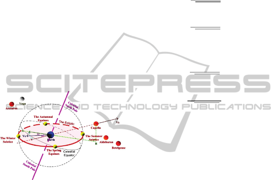
Figure 1 is a sketch of a celestial sphere and

positions of the stars. The orbital speed of the earth,

, is about 30 km/sec which is on the ecliptic plane.

Let V

denote the radial velocity of the star from the

sun and 



be the projection of the radial line of the

star on the ecliptic plane.  is the angle between V

and 



,  is the angle between V

and 



. So the

projected orbital velocity of the earth on V





. The relative radial velocity of the

star and the earth V

is 







.

Figure 1: The sketch of celestial sphere, positions of

Capella, Betelgeuse, Arcturus, Aldebaran, Vega (not on

scale), the radial velocities of Capella and the earth, and θ

and φ.

2 SYSTEM DESIGN PRINCIPLE

Some of physical parameters are dimensionless,

others are dimensional and their numerical values

depend entirely on the units in which they are

defined. The speed of light is dimensional and

expressed in terms of length per unit time. To

measure the speed of light, we need a rule and a

watch. Expecially to measure the speed of light

emitting from a moving source, we encounter the

simultaneity problem. Conventionally the detector

and the moving source are considered in two

different reference frames. In 1892, H. A. Lorentz

proposed the Lorentz Transformation as follows:

If the relative motion of the two reference frames

is along their x and x’ axes, the first frame with the

space and time units x’ and t’ moves to the right

with speed relative to the second frame with space

and time units x and t, then





()



1 











(2)





(









)



1 











(3)





= 

(4)





= 

(5)

 =

(



+ 



)



1 











(6)

 =

(













)



1 











(7)

 = 



(8)

 = 



(9)

where v is the relative speed.

In our design, we will avoid using the units

transformation and simultaneity problem. We

compare the appearent speed of starlight with the

well-known value, c. Therefore, we only use the

space and time units on the earth, in other words, we

have one rule and one clock. Also because the speed

of light is about 3 × 10



m/sec which is extremely

fast, the speed of an ordinary moving light source on

the earth is much less the speed of light. To

investigate the influence of the speed of a moving

light source on the light speed measurement is a

difficult task. However the universe provides the

experimental environment.

Our measurement system consists of a

transmitter and a distant receiver. At the transmitter,

we used a telescope to collect the light from Capella,

Betelgeuse, Arcturus, Adlebaran, and Vega. These

stars are bright and have large relative radial

velocity with respect to the earth around the Spring

Equinox. Then we modulated the starlight, terrestrial

635 nm red light, and 1550 nm infrared light into

pulses simultaneously. After travelling a distance, d,

these pulses arrived at the receiver. The red light

travelled along almost the same path of the starlight.

So we were able to use the red light and the 1550 nm

infrared pulses as the reference and trigger signals.

PHOTOPTICS2014-InternationalConferenceonPhotonics,OpticsandLaserTechnology

We used the terrestrial white light which travelled

along exactly the same path of the starlight.

If the speed of light is constant, the travelling

time of starlight pulses and the terrestrial white light

pulses from the transmitter to the receiver should be

the same as





= /

(10)

If Ritz’s assumption is valid and the speed of

starlight has deviated from the well-known value, c,

then the time taken for the starlight pulses travelling

from the transmitter to the receiver is given by





= /( 



)

(11)

where V

is the relative velocity of the star and the

earth.

3 SYSTEM DESCRIPTION

Based on the design principle and concept described

in the previous section, we have two different

designs: one using a rotating two-facet mirror and a

slit to modulate the continuous light beam into

pulses and the other employing a chopper.

3.1 The Optical System using a

Rotating Two-facet Mirror and a

Slit

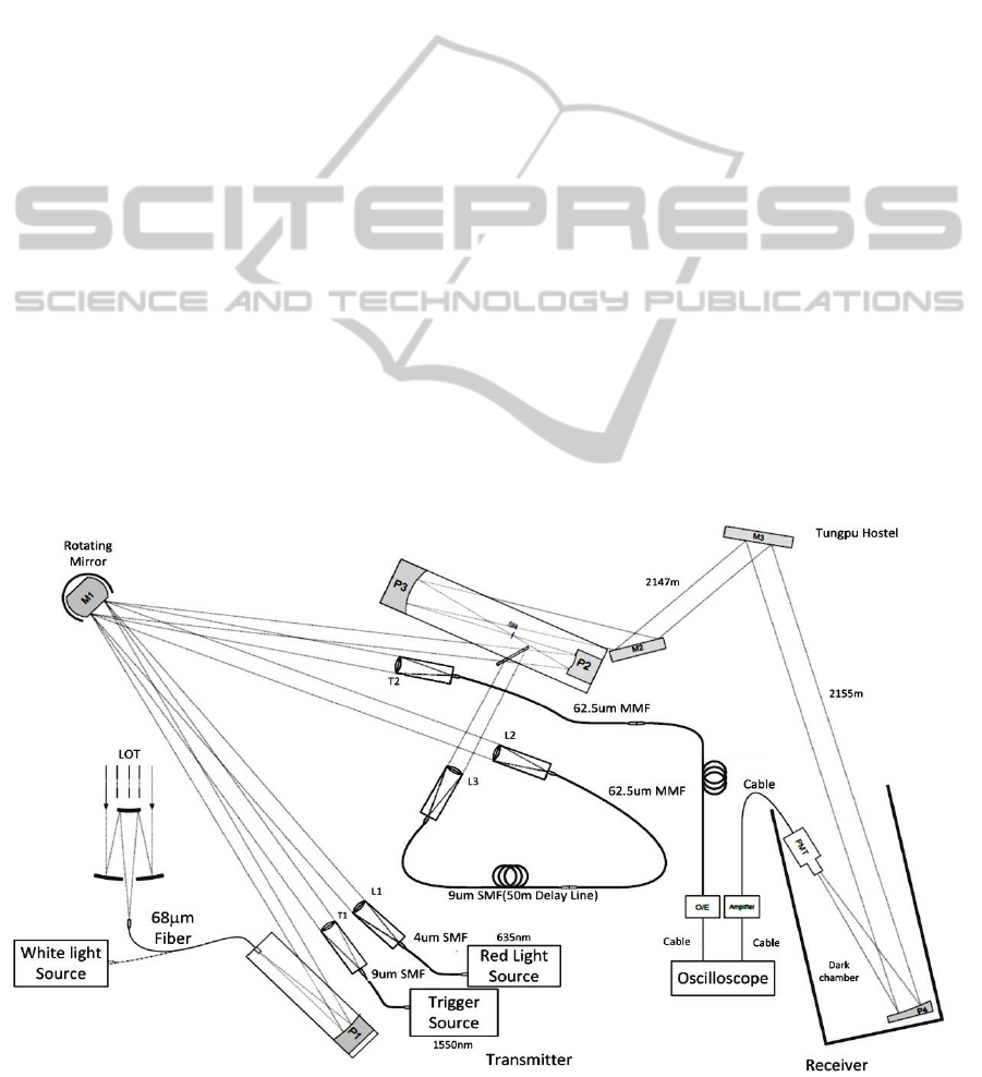
Figure 2 shows the schematics of the system layout.

At the transmitter, for the starlight path, we used the

one-meter telescope of the Lulin Observatory to

collect the starlight. One end of a five-meter fiber

with core diameter of 68 μm and the numerical

aperture about 0.0729 was placed at the focal point

of the telescope to guide the starlight. The other end

of the fiber was fixed at the focal point of the off-

axis parabolic mirror, P1, which made the ray

collimating. It was then reflected by the rotating

mirror, M1, and was incident upon the off-axis

parabolic mirror, P2. A 100 μm wide slit was located

at the focal point of P2 and another off-axis

parabolic mirror, P3. When the rotating mirror M1

spun, the light would scan across the slit to produce

light pulses. The pulses were reflected by P3 to the

planar mirrors, M2 and M3, where M3 was located

at the Tungpu Hostel about 2,147 m from the Lulin

Observatory. The collimating ray from M3 travelled

2,155 m back to the Lulin Observatory to reach the

30 cm off-axis parabolic mirror, P4. A photo-

multiplier tube (PMT) was placed at the focal point

of P4. Therefore, the total travel distance, d, was

4,302 m.

For the path of the reference red light, a laser

with a wavelength of 635 nm and a 4 μm single

mode fiber pigtail was used as the reference light

source. The end of the fiber was located at the focal

point of the lens, L1. The collimating ray from L1

was incident to the rotating mirror, M1, and then the

lens, L2, with a standard 62.5 μm multimode fiber

Figure 2: The schematics of the optical system using rotating mirror.

9um SMF

(3085 m)

TheNovelOpticalSystemofMeasuringtheSpeedofStarlight

connected a 9 μm single mode fiber located at the

focal point. The 62.5 μm fiber acted as a slit and

guided the pulses. The total length of this fiber link

was 63 meters, which separated the red light and

starlight pulses by about 300 nsec on the

oscilloscope screen when M1 spun at 17,929 rpm.

The other end of the single mode fiber of the link

was placed at the focal point of the lens, L3. Then

the collimating ray from L3 was combined with the

starlight by a beam combiner BS1. Thereafter the

red light and the starlight pulses travelling along the

same path were received by the PMT to convert

them into electrical pulses which could then be

recorded by the oscilloscope. For the trigger signal,

a 1550 nm laser with an Erbium doped fiber

amplifier and a 9 μm single mode fiber pigtail was

used as the trigger source. The end of the pigtail

fiber was placed at the focal point of the lens, T1.

The collimating ray from T1 was incident to M1 and

then the lens, T2. At the focal point of T2, we had a

standard 62.5 μm multimode fiber which acted as a

slit and guided the pulses through the 3085-meter

single mode fiber to the receiver. A photodetector

was employed to convert the infrared pulses to

electrical pulses which were used as the trigger

signal for the oscilloscope.

3.2 The Optical System Employing a

Chopper

When we use the rotating two-facet mirror and a slit

as a modulator, the reflected beam from the mirror

M1 scans over the slit to product the pulses while

the rotating mirror spun. The spindle which drives

the rotating mirror may have wobble and the angular

velocity deviation. Here we propose the optical

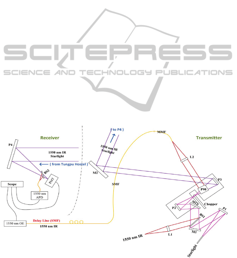
system using a chopper as the modulator. In this

system the light beam is fixed. When the chopper

spins the light beam is modulated into pulses. Figure

3 is the schematics of the optical system using a

chopper. The starlight is collected by the telescope

and guided by the 68 μm fiber whose output end is

placed at the focal point of P1. The reflected

collimating beam is incident to M1, M12 and P2.

The focal point of P2 and P3 is at the slit of the

chopper. The reflected collimating beam from P3

then is incident to the planner mirror M2 and

transmits over 4.3 km to P4. The PMT is located at

the focal point of P4. The 1550 infrared is

collimated by the lens L1 and then combined by the

beam splitter, BS1, with the starlight main path.

After the chopper, part of the 1550 nm light is

separated by the P90 beam splitter and through the

lens L2 and incident to the multimode fiber

connected to the 3.8 km single mode fiber delay line.

At the end of the single mode delay line, the

1550 nm optical/electrical converter converts the

Figure 3: The schematics of the optical system using chopper.

PHOTOPTICS2014-InternationalConferenceonPhotonics,OpticsandLaserTechnology

optical signal to the electrical signal. The rest part of

1550 nm travels along with the starlight and reaches

the receiver where the beam splitter BS2 and an

Avalanche Photon-Diode are used to separate the

1550 nm light and converts to the electrical signal.

When the chopper spins, the starlight and the

1550 nm infrared are modulated into pulses

simultaneously. The two 1550 nm pulses at the

receiver can be used as the trigger and the reference

signals. In this system, the chopper is a very

important element, which must be light weight and

easy to have dynamically balanced. We have used

titanium alloy and composite carbon fiber to

fabricate the chopper. However the preparation is

still on-going.

4 MEASUREMENT RESULTS

We used the optical system using the rotating mirror

and the slit to perform the measurement in

November 2009, March 2010, and January 2011. In

order to minimize the error due to deviation of the

spindle speed, we carefully aligned the parabolic

mirrors and the lenses P1, P2, T1, T2, L1 and L2,

such that the three beams from P1, T1, and L1, after

reflected from the rotating mirror M1, were

simultaneously incident to the slit after P2, the focal

points of T2 and L2, respectively.

Because the optical power of the starlight was

very low (in the order of a few nanowatts or less),

the PMT operated in the photon counting mode

which generated spikes instead of full waveforms.

The maximum amplitudes of dark current and

thermal noises were 0.024 volts and very small

compared to the spikes and trigger pulses. To avoid

accumulation of noises, we first choose a threshold

at 0.025 volts and set all recorded data smaller than

the threshold to zero. If there are spikes in the frame,

we classify it as a valid frame, otherwise we discard

it. To reconstruct the starlight and the red light pulse

waveforms, taking a moving average of length 100

on the trigger pulse of each valid frame, we calculate

the centroid (center of gravity) by the weighted time

average method, i.e.

centroid i i i

X XY Y=

∑∑

, where

is the sampling time and Y

is the amplitude

which is larger than 20% of the peak value. Then we

adjust the time axes of the frames by aligning the

centroids of the trigger pulses for 2,000 valid frames

and simultaneously accumulate spikes to form the

waveforms of the starlight and the red light pulses.

Because the PMT operated in the photon counting

mode, we only take the peak value of the spike

during the accumulation process. We apply Gaussian

fitting to the red light waveform to obtain the

centroid. After finishing this process for the entire

set of starlight measurement frames, we align the

centroids of the fitted red light pulses to reconstruct

the complete waveforms of the starlight and the red

light pulses. We follow the same procedure to

reconstruct the pulse waveforms of the terrestrial

white light and the red light.

Next, we again use Gaussian fitting to estimate

the centroids of the starlight, white light, and red

light pulses. We applied different fitting methods

and obtained a similar result.

In the spring of 2013, we used the similar setup

as shown in Figure 2 to measure the speed of

starlight, where we omitted the red light and used

the 1550 nm as the trigger and the reference signals.

We obtained the similar result as the previous ones.

Table 2 summarizes the average delays of the

starlight measured in 2010, 2011, 2012, and 2013.

Note that if the starlight pulses arrive at the receiver

earlier than the terrestrial white light pulses, the

delay value is negative, e.g. the Vega pulses.

The pulses of Adlebaran, Capella, and

Betelgeuse have positive delays and that of Vega

and Arcturus have negative delays. As shown in

Table 1, the relative radial velocities of Adlebaran,

Capella, and Betelgeuse are positive, but that of

Vega and Arcturus are negative. Because we had

laid the equipment on the floor of the Lulin

Observatory, the ambient temperature and the

relative humidity made the floor contraction or

expansion which affected the measurement. The

error of delays of Arcturus in 2011, Vega in 2011,

and Capella in 2012 are large.

5 CONCLUSIONS

In this paper, we presented a novel method to

measure the speeds of starlight. This method

compares the travelling times of these starlights and

the local white light from the transmitter to the

receiver. Such that physical unit transformation,

clock synchronization and definitions of dimension

units problems can be avoid. This system utilizes the

existing telescope of the observatory, the orbiting

speed of the earth, and the radial velocities of stars.

Comparing the measured apparent speeds of

Adlebaran, Capella, Betelgeuse, Arcturus, and Vega

with the well-known speed of light from a rest

source, c, we find that Adlebaran, Capella, and

Betelgeuse have positive delay, while Vega and

Arcturus have negative delay. Note that Adlebaran,

TheNovelOpticalSystemofMeasuringtheSpeedofStarlight

Table 1: The data of Capella, Betelgeuse, Arcturus, Adlebaran, and Vega.

Star Capella Betelgeuse Arcturus Vega Adlebaran

Apparent Magnitude 0.91/0.76 (B-V) 0.58 (V) -0.04 (V) 0.03 (V) 0.85 (V)

Stellar Classification G8 III / GI III M2 Iab K2 III A0 V K5 III

Right Ascension 5h16m41s 5h55m10s 14h15m39s 18h36m56s 4h35m55s

Declination +45˚59’52” +7˚24’25” +19˚10’56” +38˚47’01” +16˚30’33”

Radial Velocity V

29.65 21.91 -5.19 -13.9 54.26

Distance ( light year / parse)

42.5 ± 0.5 /

13.04 ± 0.03

643 ± 146 /

197 ± 45

36.7 ± 0.3 /

11.24 ± 0.09

25.3 ± 0.1 /

7.76 ± 0.03

65 ± 0.1 /

20.0 ± 0.4

Relative Radial Velocity ( km/sec )

( March 18, 2010 )

56.47 49.56 -20.77 -27.10 82.43

Table 2: The average delays of starlight measured in 2010, 2011, 2012 and 2013.

Delays (ns)

2010

2011

2012

2013

Adlebaran

2.40

Capella

2.28

2.41

4.57

1.20

Betelgeuse

1.19

1.80

Arcturus

-0.45

-4.01

-0.19

Vega

-1.35

-7.40

-1.20

Capella, and Betelgeuse have positive relative radial

velocity, Vega and Arcturus have negative relative

radial velocity, i.e. Adlebaran, Capella, and

Betelgeuse are leaving away from the earth and

Vega and Arcturus are approaching to the earth. The

result implies the measured apparent speed of

starlight likely relates to the relative motion of the

source and the detector.

ACKNOWLEDGEMENTS

The authors are grateful for Professor Wen-Ping

Chen, Director Hung-Chin Lin, Miss Hui-Ting Tsao

and the staff of the Lulin Observatory of National

Central University to provide the facilities and the

necessary help. This work was supported in part by

Excellent Research Projects of National Taiwan

University and the Nation Science Council, Taiwan,

under Grants 98R0062-06, NSC 100-2221-E-002-

035- and NSC 101-2221-E-002-002-.

REFERENCES

Froome, K. D., and Essen, L., 1969. The Velocity of Light

of Radio Waves, Academic Press, New York, USA.

Sanders, J. H., 1965. The Velocity of Light, Pergamon

Press Ltd., Oxford, UK.

French, A. P., 1968. Special Relativity, W. W. Norton &

Company Inc., New York, USA.

Dickey, J. O., Bender, P. L., Faller, J. E., Newhall, X. X.,

Ricklefs, R. L., Ries, J. G., Shelus, P. J., Veillet, C.,

Whipple, A. L., Wiant, J. R., Williams, J. G., and

Yoder, C. F., 1994. Science 265, 482.

Anderson, J. D., Laing, P. A., Lau, E. L., Liu, A. S., Nieto,

M. M., and Turyshev, S. G., 1998. Phys. Rev. Lett. 81,

2858.

Ritz, W., 1908. Amn.de Chim, et de Phys. 13, 145-275.

Torres, G., Claret, A., and Young, P. A., 2009. Astrophys.

J. 700, 1349.

Wilson, R. E., 1963. General Catalogue of Stellar Radial

Velocities, Carnegie Institution of Washington

Publication, Washington, D. C., USA.

SIMBAD Astronomical Database, from http://simbad.u-

strasbg.fr/simbad/.

Wu, J., Chang, S. -T., Tsao, H. -W., Huang, Y. –R., Lee, S.

-L., et al., 2012. Testing the Constancy of the velocity

of Light. Am. Phy. Soc. April Meeting. Atlanta, USA.

Huang, Y. -R., Wu, J., Lin, W. -C., Chang, S. -T., Lee, S. -

L., Tsao, H. -W., et. al., 2012. An Optical System of

Comparing the Speeds of Lights from Moving Stars.

ODF 12. Saint-Petersburg, Russia.

Wu, J., Chang, S. -T., Tsao, H. -W., Huang, Y. -R., Lee, S.

-L., et. al., 2013. A Method of Comparing the Speed

of Starlight and the Speed of Light from a Terrestrial

Source. SPIE Optics + Photonics 2013. San Diego,

USA.

Huang, Y. -R., Wu, J., Chang, S. -T., Tsao, H. -W., Lee, S.

-L., and Lin, W. -C., 2013. Measurement of

Differences and Relativity between Speeds of Light

from Various Stars. APPC 12. Chiba, Japan.

PHOTOPTICS2014-InternationalConferenceonPhotonics,OpticsandLaserTechnology