In-wall Thermoelectric Harvesting for Wireless Sensor Networks

Aristotelis Kollias and Ioanis Nikolaidis

Computing Science Department, University of Alberta, Edmonton, T6G 2E8, Alberta, Canada

Keywords:

Wireless Sensor Networks, Energy Harvesting, Thermoelectric Energy.

Abstract:

We propose the use of embedded in-wall thermoelectric harvesters to power nodes of a wireless sensor net-

work. We exploit the signiﬁcant temperature differences between indoor and outdoor environments in cold

climates. We use heat ﬂow measurements of the exterior (outside-facing) wall of a number of apartments

from the same apartment complex. We report on the degree of variability as well as on the seasonal changes

that characterize the heat ﬂow, and hence the potential for thermoelectric energy harvesting. We also exam-

ine whether the difference between indoor and outdoor air temperature is a good proxy for to the observed

heat ﬂow through the walls. Examples of data carrying capability of a particular harvester and sensor node

combination are also provided.

1 INTRODUCTION

Wireless sensors are used to assist in structure main-

tenance (Vullers et al., 2010), to monitor human ac-

tivity, to help prevent disasters like forest ﬁres, and,

in general, to collect data for scientiﬁc and business

purposes. In the construction industry, sensors can be

used to alert of dangerous situations, in cases where

the infrastructure is critically compromised and to

monitor wear and the “health” of buildings in gen-

eral. For example, humidity sensors inside wall struc-

tures can provide advance warning of excess humidity

which could lead to toxic mould growth, and strain

dynamometers sensors can be used to determine the

response of the building during earthquakes.

We consider the standard model for wireless sen-

sor network (WSN) nodes, i.e., as consisting of a

transceiver, the sensor, a microcontroller and an en-

ergy source, usually a battery. Generally, when the

energy source for the WSN node is a battery, there

exists a limit to how long the node can function with-

out servicing, i.e., changing of batteries. With current

technology, the node modules generally exhibit low

energy consumption, therefore the lifetime limit that

a battery imposes can be long enough that, depending

on the situation, replacing batteries will not impose a

signiﬁcant cost. However, in particular situations, the

sensors are inaccessible, i.e., embedded within struc-

tures, like walls, and the cost of replacing the energy

source might be prohibitive.

There are three possible solutions for difﬁcult–to-

access sensor nodes. They can be either abandoned

after they have performed their function for some time

(with the hope that other, nearby, sensors will take

over the task of measuring the same phenomenon),

or they can be all connected to a wired power distri-

bution subsystem. Finally, energy harvesting could

be employed. Abandoning the sensors is an expen-

sive option and possibly unacceptable. The wiring

option is expensive in terms of labor cost and mate-

rials, exacerbated by the ever increasing price of cop-

per, and wiring defeats the advantage of using wire-

less, since communication can be accomplished over

the same wires that provide power. Wiring also re-

sults in a structure which is more complex and could

be prone to faults (accidental puncture/cutting of the

wires, problems with single points of failure, collec-

tion of RF energy by acting as low frequency anten-

nas, etc.). In short, the ability of each node to power

itself from energy harvesting leads to better node au-

tonomy, and overall system resilience.

The solution adopted in this paper is to use ther-

moelectric energy harvesters to power each sensor

node. Energy harvesters exploit the ambient energy of

the environment to replenish the energy stored in the

battery or the super capacitor. Photovoltaic harvesters

have been studied extensively in previous works e.g.,

(Gorlatova et al., 2011). Buildings with good illumi-

nation can use photovoltaic energy to power sensor

modules. Instead, in this paper we consider thermo-

electric energy harvesting because (a) the potential for

photovoltaic energy can be limited due to sub-optimal

213

Kollias A. and Nikolaidis I..

In-Wall Thermoelectric Harvesting for Wireless Sensor Networks.

DOI: 10.5220/0004864102130221

In Proceedings of the 3rd International Conference on Smart Grids and Green IT Systems (SMARTGREENS-2014), pages 213-221

ISBN: 978-989-758-025-3

 2014 SCITEPRESS (Science and Technology Publications, Lda.)

placement, and because of long nights, as is the case

at latitudes of northern continental climates, while,

(b), during winter the indoor to outdoor temperature

difference can reach as much as 60 degrees Celsius

creating unparalleled opportunities for thermoelectric

harvesting. More speciﬁcally, we take advantage of

the difference between indoor and outdoor tempera-

ture in buildings in northern climates. To this end, we

use data collected from an actual inhabited apartment

complex in Fort McMurray, Alberta, Canada. The

particular apartment complex has been constructed

using modular construction techniques.

Placing thermoelectric harvesters inside walls

serves the application of powering co-located sensors

that monitor the wall and building behaviour. In cli-

mates like the one considered in our study, extreme

weather conditions can cause events important to the

integrity of a building, e.g., breakage of water pipes,

more frequently occurring than in moderate climates.

The ability to embed sensors in inaccessible locations

that autonomously operate for several decades (i.e., as

long as the building lasts), monitoring for such events,

can currently only be supported using energy harvest-

ing.

In terms of the methodology followed, we use the

difference between indoor air and outdoor air temper-

ature as the basis for the energy harvesting potential

we report in this paper. Nevertheless, the energy har-

vesting speciﬁc to an apartment (and, more speciﬁ-

cally, to a location on an exterior wall of an apart-

ment) depends on a number of factors whose com-

bined effect can be captured by the heat ﬂow rate

through speciﬁc locations of the exterior walls. We

therefore study whether the difference between indoor

and outdoor temperature at each apartment is a good

proxy for the actual heat ﬂow via the exterior walls.

The heat ﬂow is the real rate of energy transfer via the

wall unit, i.e., the ground truth. Our study indicates

among other things that, even though the difference

between indoor and outdoor air temperature is a good

(scaled) proxy for the average heat ﬂow, there exists

a high degree of variability of heat ﬂow across apart-

ments. Furthermore, the variability is smaller during

certain times of the year. We comment on how these

observations should guide the design of suitable net-

work protocols.

The remaining of the paper is structured as fol-

lows. Section 2 brieﬂy reviews some related work on

the subject at hand, Section 3 has the description of

the data set, and elements of the methodology we fol-

lowed in interpreting them. Section 4 outlines the sys-

tem model that we employ. Section 5 presents numer-

ical performance results. We conclude with Section 6

summarizing our ﬁndings.

2 RELATED WORK

Energy harvesting for wireless networks and low

power wireless sensor node architectures are areas of

intense research activity. The use of energy harvesting

for powering WSN nodes, with example applications,

such as smart buildings and predictive maintenance of

structures has been explored in the past (Vullers et al.,

2010).

In this paper we narrow our focus to thermoelec-

tric generators and speciﬁcally exploit the energy lost

through walls in cold climates. We use a device model

loosely based on (Mateu et al., 2006), in which energy

harvesting from the human body was used, which is

an idea explored by other researchers as well, (Ra-

madass and Chandrakasan, 2011; Wang et al., 2009).

The devices proposed in previous works assume oper-

ation based on the difference of temperature between

the human body and its environment, thus indirectly

exploiting the temperature homeostasis of the human

body.

In this paper, we are not concerned with the task of

increasing the energy harvesters efﬁciency, a topic of

intense activity anyway, e.g., (Hudak and Amatucci,

2008; Luber et al., 2013). We use off-the-shelf com-

ponents and we do not even use a sensor platform op-

timized for energy efﬁciency. In other words, the re-

sults we present here are very close to representing a

“worst case” scenario with respect to the devices em-

ployed.

In the ﬁeld of energy harvesting for WSNs, a no-

table work is that of Gorlatova et al. (Gorlatova et al.,

2009; Gorlatova et al., 2011) which focuses on how

to use photovoltaic harvesting under diverse use sce-

narios, by proposing suitable optimization models.

Another distinct property of their work is the study

of photovoltaic harvesting in environments under the

control of the users (depending on indoor illumina-

tion, or in the pocket of users), i.e., with idiosyncratic

and sometimes unpredictable behaviour. They also

consider elementary WSN applications, such as ID

beacon transmission.

3 THE DATA SET

We use data collected over a period of a year, from 11

different apartments within a single apartment com-

plex in Fort McMurray, Alberta, Canada. The data

collected is comprehensive, including such aspects as

water ﬂow and temperature for the water used by radi-

ators for heating, water ﬂow and temperature for res-

idential water, CO2 concentration, etc. For the pur-

poses of this study we consider only the heat ﬂow

SMARTGREENS2014-3rdInternationalConferenceonSmartGridsandGreenITSystems

214

through exterior (outside-facing) walls, the indoor air

temperature, and the outdoor air temperature. The

data collection was conducted in real–time and is still

taking place, but we extract a one year period (8th of

September of 2012 to the 8th of September of 2013)

which is sufﬁcient for the purposes of capturing sea-

sonal variations.

In our data set, we obtain a separate indoor air

temperature for each apartment but have a single out-

door air temperature, as acquired by the Building Au-

tomation System (BAS). It has to be noted that a sin-

gle outdoor air temperature is, again, only an approx-

imation of the locally speciﬁc outdoor wall temper-

ature of each wall unit, since phenomena like con-

vection can, depending on airspeed, result in different

temperatures at different spots and orientations.

The heat ﬂow measurements are obtained at two

locations (one on a stud, and one on the insulation)

of the exterior–facing wall of each apartment. Of the

two heat ﬂow measurements the one most relevant to

our study, which we subsequently use, is the heat ﬂow

via the stud. Studs are necessary for the structure and

proper framing of the walls but at the same time they

are responsible for loss of heat as they represent a

“bridge” of smaller thermal resistance (compared to

the insulated area of the wall) between interior and

exterior.

3.1 The Methodological Approach

The heat ﬂow through a wall reﬂects the combined

results of wall construction qualities (stud spacing,

insulation, etc.), of human activity (e.g. the choice

of thermostat setpoints, opening of windows, etc.),

of weather phenomena (temperature, wind direction,

etc.), the particular orientation and location of the

apartment, and of course the exact location of the sen-

sor in the wall. As we will see, the combination of the

factors leads to a highly variable heat ﬂow which nev-

ertheless exhibits distinct seasonal characteristics.

We use heat ﬂow data to describe the extent to

which thermoelectric energy harvesting through the

exterior walls is adequate to power (and to what de-

gree) WSN nodes. Heat ﬂow (measured in W /m

units) through exterior walls is directly related to the

temperature difference between the two sides of the

wall. Heat ﬂow through an inﬁnitesimally narrow

slice of surface is deﬁned as, ~q = −k∇T where ~q is

the local heat ﬂow, k is the materials heat conductivity

and ∇T is the temperature gradient. We note that heat

ﬂow is a vector. We use the convention that a positive

heat ﬂow represents loss of heat (i.e., radiating from

the interior side of the wall to the exterior side) while

a negative indicates the reverse direction. Naturally,

due to the climate characteristics in Fort McMurray,

the latter case is infrequent, and occurs almost exclu-

sively during the warmest summer months.

More precisely, if the wall is to be treated as a sin-

gle homogeneous material of inﬁnite area and thick-

ness L the heat ﬂow is inversely proportional to the

thickness, that is, ~q = −kL

−1

∇T . In reality, the walls

are more complex non-homogenous structures con-

taining cavities, insulation, studs for wall support,

studs for window framing, etc. impacting collectively

on the heat ﬂow magnitude and direction.

The thermoelectric harvesters are also dependent

on the temperature differences to produce electricity

and their output is governed by −∇V = S∇T where

S is the Seebeck coefﬁcient of the material and ∇V

is the electric potential between the two harvester ter-

minals. In Section 5 we correlate the heat ﬂux data

h f

) with the air temperature difference between in-

door and outdoor (∆T

air

After establishing a strong relation between q

h f

and ∆T

air

, we subsequently use ∆T

air

as a proxy of

the actual temperatures of the two (inside and outside)

wall surfaces. This is primarily because the air tem-

perature represents averages whereas q

h f

is speciﬁc

to the location of the wall where the heat ﬂow sen-

sor is mounted. However, our reasoning is that any

thermal harvester installed in the wall will experience

similar heat transfer behaviour as the heat ﬂow sen-

sors measure at the same location. Hence, whereas

∆T

air

is a good basis for an overall estimate of en-

ergy harvesting potential, regardless of where the har-

vester is placed on the exterior wall, q

h f

allows us to

examine the highly idiosyncratic behaviour (captured

by the standard deviation) due to the factors we listed

at the beginning of this section.

Our interest in ∆T

air

and q

h f

and their relation is

also motivated by the intention to use, in a future de-

sign, a thermoelectric harvester inside the wall whose

two sides are in contact to the two wall surfaces via

materials of high thermal conductivity, e.g., metal.

This would allow the thermal harvester to be a low

thermal resistance “bridge” and hence receive the full

potential of the temperature difference of the two sur-

faces. However, such a design is future work because

it needs to satisfy several other structural, mechanical,

and safety constraints for in-wall embedding.

4 THE DEVICE MODEL

4.1 The Harvester Model

Our model is based on the performance of the TEC1-

12703 Peltier module. The module has a surface area

In-WallThermoelectricHarvestingforWirelessSensorNetworks

215

of 16 cm

. We carried out characterization experi-

ments to determine the relation between ∆T and en-

ergy harvested. The setup was a small “refrigerator”,

using TEC1-12703 modules (see Figure 1), arranged

such that, a constant ∆T was created and the result-

ing energy harvested measured. This refrigerator is

made by using (top to bottom): (i) a heat sink, which

is connected to a TEC1-12703, also connected to a

power supply, to provide the hot side temperature for

the harvester, (ii) the harvester, with its other side con-

nected to, (iii) another TEC1-12703 module, again

connected to the power supply to provide the cold side

temperature. Lastly, another heat sink along with a

small fan was used to help regulate the heat and stabi-

lize ∆T. This setup was used to maintain constant ∆T

ranging up to 40 degrees Celsius. The temperatures

were sensed using thermistors, and a separate sensor

module. Our ﬁndings indicate that the power output,

W (in mW ), of the particular harvester relates to ∆T

(in Celsius) as W = (2.57 ∆T

+ 5.88 ∆T + 0.11) ·

−3

(Least Squares ﬁt with R

= 0.9358).

4.2 The Sensor Model

In order to develop a WSN node energy consumption

model, we use the NanoZ-CC2530 device which em-

ploys the TI CC2530 microcontroller. We operate it

with another node acting as data sink, communicating

using the z-stack tool (ti.com, 2012) (Zigbee compli-

ant). We carried out energy-exhaustion tests to deter-

mine for how long (how many bytes) of payload can

be transmitted for the amount of energy accumulated

to sufﬁciently charge a 1 Farad capacitor (rated at 5V )

up to 3.6 V. The packets transmitted followed the

standard Zigbee data frame structure. We ﬁrst con-

ducted experiments using the TEC1-12703 harvester

connected to a Texas Instruments BQ25504 Evalua-

tion Board to regulate the voltage and to determine

the ability of the harvester to charge the capacitor.

After the success of the ﬁrst step, and in the interest

of accelerating the experiments, we used a standard

power supply (GPC-3030) to charge the capacitor to

the same 3.6V . The capacitor was then connected to

the NanoZ module and used to send data until exhaus-

tion. From the measurements we concluded that it

was possible to transmit an average of 4103.7 bytes of

payload per Joule using messages of maximum pay-

load size (90 bytes per packet). The sensor modules

are not energy efﬁcient, as we measured that they con-

sume 0.49 mW in their sleep state when the processor

is set to the sleep mode PM2 (only low-frequency os-

cillator operating), of which only approximately 6µW

is due to the processor consumption (as per the pro-

cessor datasheet).

Figure 1: The harvester experimental setup. Shown in the

ﬁgure are: (a) heat sink for temperature control of the “hot

side”, (b) thermistor for measuring the “hot side” tempera-

ture, (c) thermoelectric heater for the hot side, (d) the ther-

moelectric harvester, (e) the same as (c) but for generating

the “cold side” temperature, (f) fan with heat sink for ther-

mal control of the “cold side”.

Table 1: Correlation of ∆T

air

and q

h f

Apartment corr(∆T

air

h f

)

1 0.86

2 0.93

3 0.90

4 0.82

5 0.81

6 0.88

7 0.85

8 0.91

9 0.84

10 0.86

11 0.84

5 NUMERICAL RESULTS

We ﬁrst consider the correlation of the ∆T

air

and q

h f

time series over the entire year and separately for each

apartment. The time series represent hourly averages

of the respective values. Table 1 demonstrates the

overall strong correlation of the two time series but

there exist differences (e.g. 0.93 for apartment 2 and

0.82 for apartment 4) that are ultimately related to the

occupant(s) actions and behaviour. To illustrate the

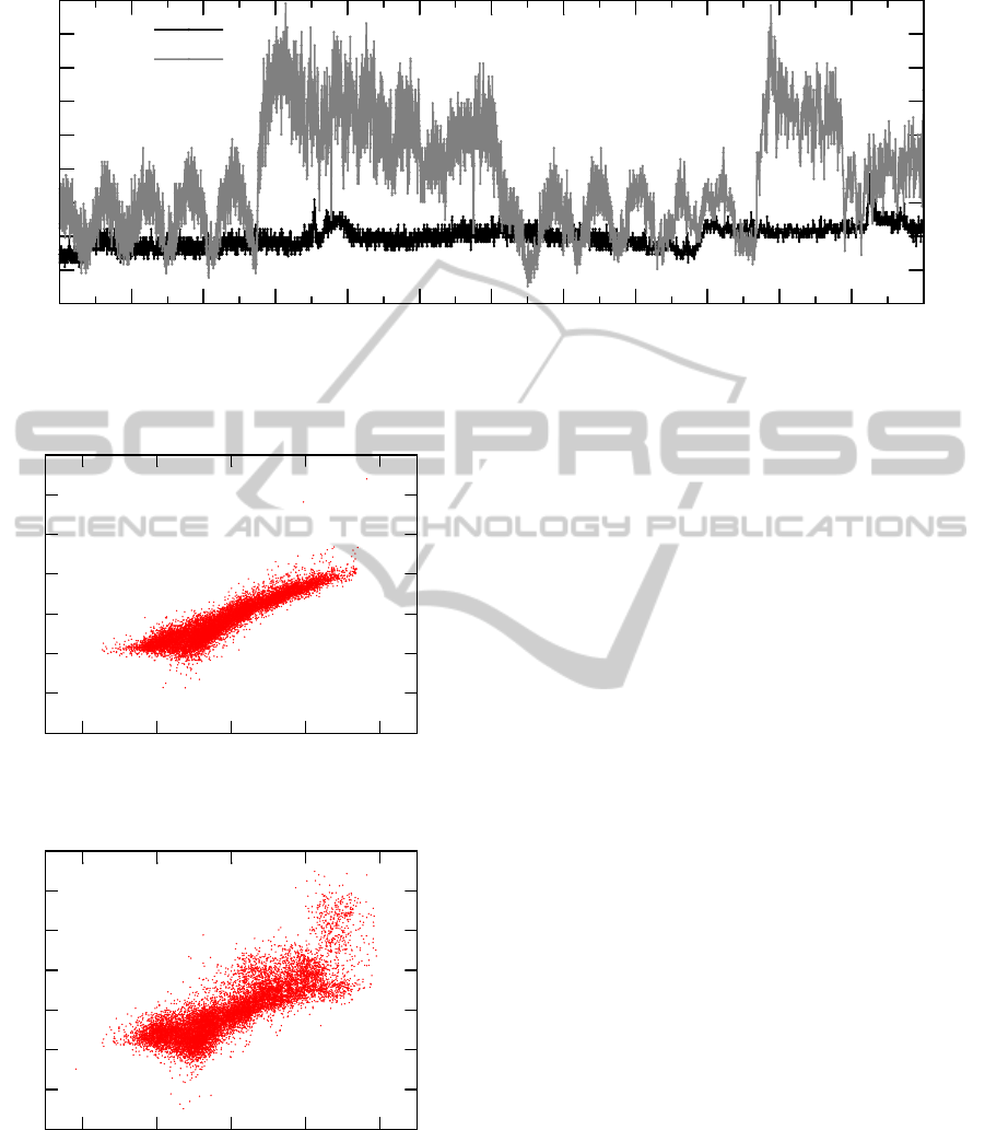
nature of differences consider the scatterplots of ∆T

air

and q

h f

in Figure 3 and 4 for the entire year, show-

ing an overall strong correlation but with signiﬁcant

SMARTGREENS2014-3rdInternationalConferenceonSmartGridsandGreenITSystems

216

00:00

02:00

04:00

06:00

08:00

10:00

12:00

14:00

16:00

18:00

20:00

22:00

00:00

APT 2

APT 4

h f

(W /m

)

Figure 2: Intra-day q

h f

in apartments 2 and 4.

-10

-5

-20 0 20 40 60

∆T

air

(C)

h f

(W /m

)

Figure 3: Apartment 2 ∆T

air

vs. q

h f

-10

-5

-20 0 20 40 60

∆T

air

(C)

h f

(W /m

)

Figure 4: Apartment 4 ∆T

air

vs. q

h f

variance and occasional outlier points.

Without precisely knowing the inhabitants be-

haviour, one can only conjecture on several reasons

for certain outliers (the resident could have been us-

ing an electrical radiator close to the location of the

heat ﬂow sensor, or touching the wall at the sensor

location, or had the windows open, etc.). To illus-

trate the differences that might show up, consider Fig-

ure 2 showing the heat ﬂow during a speciﬁc day (in

mid-March of 2013) during which one of the two pre-

sented apartments had almost constant heat ﬂow (pos-

sibly the apartment was vacant that day) while the

other one had highly variable heat ﬂow (the oscilla-

tions are probably due to the heating cycling around

the thermostat setpoint, while higher setpoints and

possible resident activity are evident from approxi-

mately 6am to 12pm and from approximately 8pm to

10pm).

We deﬁne s

(d)

avg

, s

(d)

max

, and s

(d)

min

as, respectively, the

average, maximum, and minimum of daily q

h f

stan-

dard deviation, calculated based on the hourly mea-

surements of each day. Essentially we try to cap-

ture the statistics of variability of q

h f

within the same

day as they behave across the year. As can be seen

from Table 2 the remarkable fact is that there exist

days that almost every apartment shows a drastically

small standard deviation. Apartments 3 and 4 exhibit

a s

(d)

min

of 0.18 and even the apartment 11 which has

the largest intra-day standard deviation of 8.37 still

has low variability days as its s

(d)

min

of 0.37 illustrates.

Our current conjecture is that the days of low vari-

ability represent days that the apartments were pos-

sibly vacant, and hence no resident–related inﬂuence

was introduced apart from leaving the thermostat at a

particular (and possibly low) setpoint.

Next, we try to capture the differences across

groups of apartments based on the ﬂoor and their ori-

entation. To this end, we deﬁne σ

(y)

avg

, σ

(y)

max

and σ

(y)

min

representing, respectively, the average, maximum and

In-WallThermoelectricHarvestingforWirelessSensorNetworks

217

Table 2: q

h f

and its standard deviation for various apartments, and potential harvesting output.

Apt. avg.q

h f

(d)

avg

(d)

max

(d)

min

harvested (mW ) bytes/day

1 7.19 1.70 5.17 0.31 2.15 761864(588130)

2 5.91 0.98 2.76 0.19 1.74 617129(443395)

3 8.31 1.82 5.76 0.18 2.58 916274(742539)

4 6.80 2.06 6.42 0.18 2.06 730854(557119)

5 6.50 1.84 6.55 0.34 2.30 815768(642034)

6 8.25 2.64 7.20 0.41 2.23 790079(616345)

7 5.61 2.46 6.77 0.48 2.11 747428(573694)

8 8.07 1.40 4.15 0.26 2.45 870314(696580)

9 7.30 2.74 5.79 0.29 2.28 809130(635396)

10 6.85 3.24 7.99 0.42 2.06 730610(556876)

11 7.18 2.15 8.37 0.37 1.91 675688(501954)

minimum of the standard deviation of the daily av-

erages of particular groupings of apartments across

the entire year. Table 3 (ε stands for a quantity less

than 0.005) provides some interesting results. As ex-

pected, by comparing to Table 2, the overall variabil-

ity is less pronounced at the larger time scale of a year

as it dilutes the effects of intra-day variance seen in

Table 2. While the maximum variability, i.e., σ

(y)

max

can still reach signiﬁcant levels, it is less than the one

observed intra–day.

The minimum, σ

(y)

min

, reaches a small value which

occurs during summer days when the outdoor and in-

door temperatures are almost equal and the temper-

ature across all apartments is similar as well. Un-

fortunately, less variable days across apartments are

also days of small harvesting potential because ∆T is

small. Furthermore, due to the occupant behaviour,

we encounter cases such as the average q

h f

at ﬂoor 3

and 4 being quite different (6.66 vs. 7.41). The im-

plication of this observation is that, should multi-hop

forwarding be used in the sensor nodes, the bottle-

neck (in terms of nodes with least harvested energy)

could assume undesirable topological characteristics,

by restricting the paths that could be followed to col-

lect the data to sink nodes. In this example, an entire

ﬂoor may not have enough energy to forward trafﬁc

between adjacent ﬂoors, towards a sink node placed

at the bottom ﬂoor.

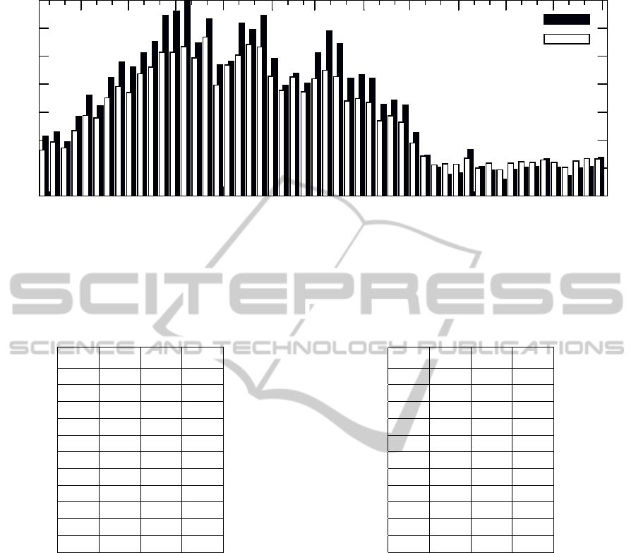
Despite the variability, seasonal patterns are evi-

dent across all apartments. Consider for example Fig-

ure 5 which shows the differences of two apartments

(number 2 and 4) over the entire year. Indeed, even

though the differences on certain days can be signiﬁ-

cant, they follow identical seasonal trends. The trends

are also similar to all the other apartments (not shown

here for the sake of brevity).

Finally, we note that there exist relatively impor-

tant differences in the heat ﬂow, and hence on harvest-

ing potential, between night and day. To put it dif-

Table 3: Average q

h f

vs. orientation/elevation.

avg.q

h f

(y)

avg

(y)

max

(y)

min

Orientation

North 7.00 0.95 3.08 0.17

South 7.14 0.78 3.04 0.24

Elevation

1st ﬂoor 7.05 0.25 4.19 ε

2nd ﬂoor 7.22 0.78 3.57 0.11

3rd ﬂoor 6.66 0.74 3.02 0.03

4th ﬂoor 7.41 1.06 4.18 0.02

ferently, the amount of energy collected in the morn-

ing hours is generally different from what could be

collected overnight. Therefore, the intra–day vari-

ability could be handled by collecting energy over

an entire (and possibly more than one) day, modulo

of course the seasonal variations. For the night vs.

day differences, we present the, rather arbitrarily cho-

sen, intervals of day (6am to 6pm) and night (6pm to

6am). Hence, each day represents two (average) mea-

surements. When considered in groupings of weeks,

and across all weeks of the year, we produce Table 4

where we can readily see the ratio between maximum

and minimum standard deviation can be signiﬁcant

and it is not uncommon to ﬁnd a 5-times difference

(apartment 6 is a good example with maximum over

a week of 4.09 and minimum over another week of

0.77). Extending the averaging over a longer time

scale will naturally smooth the variability extremes.

For example, in Table 5, each entire day is represented

by its average value, and the standard deviation of the

daily measurements over a month (deﬁned as a se-

quence of 30 days) are reported, across the entire year.

The maximum variability is tamed but the difference

between minimum and maximum standard deviation

of the same apartment can still be surprisingly large

(apartment 6 has a maximum of 3.09 and a minimum

of only 0.30).

SMARTGREENS2014-3rdInternationalConferenceonSmartGridsandGreenITSystems

218

10/01/2012

11/01/2012

12/01/2012

01/01/2013

02/01/2013

03/01/2013

04/01/2013

05/01/2013

06/01/2013

07/01/2013

08/01/2013

09/01/2013

APT 4

APT 2

h f

(W /m

)

Figure 5: Daily average q

h f

in apartments 2 and 4.

Table 4: Average, maximum and minimum weekly standard

deviation of q

h f

Apt. s

(w)

avg

(w)

max

(w)

min

1 1.25 2.28 0.48

2 0.87 1.51 0.29

3 1.51 3.21 0.37

4 1.50 3.17 0.49

5 1.24 3.25 0.47

6 1.97 4.09 0.77

7 1.38 2.31 0.49

8 1.37 2.79 0.49

9 1.93 2.91 0.79

10 1.97 3.54 0.70

11 1.53 3.17 0.61

5.1 Data Transfer Capabilities

Let us return to Table 2 and notice the harvested

power potential using ∆T

air

and the model of the har-

vester noted earlier. The average power that can be

harvested in the apartments exterior wall is 2.17 mW

with a standard deviation of 0.22 mW . The highest

average is 2.58 mW , and the apartment producing the

lowest could harvest 1.74 mW . Assuming we har-

vest energy to transmit once a day, each node could

transmit an average of approximately 770 kbytes of

payload per day. The per-apartment potential daily

transfer volume can be seen in Table 2. The numbers

in parentheses are the payload that could be trans-

mitted per day assuming at all other times the sen-

sor node idles as described in the node model, i.e.,

consuming 0.49 mW in its sleep state. Admittedly,

much better performance is possible with better de-

Table 5: Average, maximum and minimum monthly stan-

dard deviation of q

h f

Apt. s

(m)

avg

(m)

max

(m)

min

1 1.40 2.27 0.81

2 0.93 1.57 0.40

3 1.52 2.44 0.68

4 1.44 2.34 0.62

5 1.17 1.79 0.35

6 1.89 3.09 0.30

7 1.44 2.17 0.44

8 1.47 2.36 0.48

9 1.80 2.61 0.18

10 1.99 2.76 1.22

11 1.57 2.65 0.62

signed nodes. However, even at 600 kbytes of payload

per day, a sensor can adequately send samples of its

own sensing (e.g.. slowly changing humidity values

or accelerometer activity compressed to the interest-

ing events only) and still have some energy capacity

to perform multi-hop routing.

However, as Figure 5 indicates, during the sum-

mer there might not be enough power to send data

without risking an outage. Speciﬁcally, apartment 11

during the week of 6/29 to 7/5 was able to harvest

only an average power of 0.113 mW , that is not suf-

ﬁcient to even power the sensor module. The exact

sensor node design is also important. For example,

assuming that an external circuit duty-cycles the oper-

ation of the entire node, then the restarting (equivalent

to a cold boot) of the particular nodes we employed

takes around 2 seconds to complete during which

time it consumes the same power as when transmit-

ting, 84.51 mW . After those 2 seconds the device en-

In-WallThermoelectricHarvestingforWirelessSensorNetworks

219

ters sleep mode where it consumes 0.49 mW . Hence,

power-up is a costly overhead of ∼ 169.02 mJoule,

and a strategy of repeatedly powering up on-demand

to gather data (not even transmitting) is probably un-

acceptable. Or, equivalently, the particular sensor

would have to harvest energy for an average of 1497

seconds, to just cope with the 2 seconds startup energy

cost before it performed any useful sampling, com-

putation, and transmission (energy permitting), thus

limiting the rate of sampling/sensing.

If the energy storage capacity is small to allow

the longer term harvesting, outage is almost certain

during summer months. The particular apartments do

not have air-conditioning units for cooling, as they are

rarely used in such northern climates. Thermoelectric

harvesting during the summer occurs mostly at night

when the outside temperature drops.

The good news is that due to the signiﬁcant vari-

ability across apartments and throughout the day, a

protocol to determine, at least locally, which node has

(or has had in the recent past) the good fortune of har-

vesting more energy could be suitable for routing. In

other words, there indeed exists diversity of oppor-

tunities to spend energy of another neighboring node

because of the corresponding diversity in inhabitant

behaviour. As a rule though, such routing strategies

must become more conservative during the summer

when the harvesting potential is reduced in both abso-

lute numbers and in terms of variability across apart-

ments. Our recommendation would therefore be in

favour of “seasonally-aware” routing algorithms.

The potential of photovoltaic output from a cell of

the same surface area (16 cm

) as the thermoelectric

harvester used, at the same geographical location, and

using off-the-shelf solar cells with efﬁciency 17% on

a south-facing vertical wall is an average daily power

of 88.739mW (according to data in Natural Resources

Canada website (pv.nrcan.gc.ca, 2013). The average

power from thermoelectric harvesting appears low by

comparison. However, one has to consider that (1) the

solar power favors the south facing side of the build-

ing, over the north facing ones, and (2) to harvest solar

energy the placement of the photovoltaic cells is cru-

cial and one has to consider problems of occlusion of

the light source, compared to a fairly ﬂexible place-

ment of the thermoelectric harvesters. Finally, as a

matter of aesthetics, a photovoltaic harvester requires

that it be exposed to outside view, whereas a ther-

moelectric harvester can be embedded “out of sight”

within the wall structures.

6 CONCLUSIONS

In anticipation of deploying in-wall wireless sensors

for structure monitoring this paper reports measure-

ments of temperature difference and heat ﬂux taken

in an apartment building at Fort McMurray, Alberta,

to evaluate the feasibility of using thermoelectric en-

ergy harvesting in cold northern climates. We con-

clude that the use of such harvesters for wireless sen-

sor modules is possible with current technology albeit

not without some challenges.

First, even though the difference between indoor

and outdoor air temperature is a good proxy for the

potential energy harvesting, the exact behaviour of

heat ﬂow that ultimately governs the thermoelectric

harvesting at particular points of the wall structure

are subject to factors that are dependent on weather

phenomena (e.g., convection phenomena on the wall

surfaces) but, more importantly, on the behaviour pat-

terns of the residents who are in control of not only

the thermostat setpoints but also of objects attached

to or close to the walls, extra forms of directional heat

radiators (e.g. electric heaters), and so on.

Second, even though the heat ﬂow follows, as ex-

pected, a seasonal pattern, its variability from one out-

side wall to another (one apartment to another) can be

signiﬁcant, especially when observed in small time

scales, e.g., intra-day. Hence, despite the regularity

of the harvesting potential, it is to be expected even

within the same day, that the wall on some apart-

ments can sustain higher volume of sensor data trans-

fers than others. The implications of this behaviour to

multi-hop routing are obvious. Short-term alternative

routing paths would need to be considered.

Finally, the harvesting potential is reduced in the

summer months and appears possible almost exclu-

sively later in the day. Additionally, in the summer

months, the variability of harvesting becomes smaller.

Hence, sizing the energy storage (e.g., capacitance of

a supercapacitor) necessary to sustain the sensor node

operations, should be based on the worst case sum-

mer harvesting potential. One could argue that we

need to consider complementing thermoelectric har-

vesting with photovoltaic harvesting which reaches its

peak output during the summer months. Nevertheless,

such a decision is dependent on a decision to expose

the photovoltaic element which we try to completely

avoid as we wish to deploy the sensors as inconspicu-

ously as possible.

We are currently working towards a modular de-

sign for simple in-wall placement.

SMARTGREENS2014-3rdInternationalConferenceonSmartGridsandGreenITSystems

220

ACKNOWLEDGEMENTS

The authors would like to thank the funding sup-

port of the Natural Sciences and Engineering Re-

search Council of Canada (NSERC) through a CRD

Grant and the invaluable technical assistance of Mrs.

Veselin Ganev and Jianfeng Dai.

REFERENCES

Gorlatova, M., Kinget, P., Kymissis, I., Rubenstein, D.,

Wang, X., and Zussman, G. (2009). Challenge: ultra-

low-power energy-harvesting active networked tags

(enhants). In Proceedings of the 15th annual interna-

tional conference on Mobile computing and network-

ing, pages 253–260. ACM.

Gorlatova, M., Wallwater, A., and Zussman, G. (2011). Net-

working low-power energy harvesting devices: Mea-

surements and algorithms. In INFOCOM, 2011 Pro-

ceedings IEEE, pages 1602–1610.

Hudak, N. S. and Amatucci, G. G. (2008). Small-scale en-

ergy harvesting through thermoelectric, vibration, and

radiofrequency power conversion. Journal of Applied

Physics, 103(10):101301–101301.

Luber, E. J., Mobarok, M. H., and Buriak, J. M. (2013).

Solution-processed zinc phosphide (α-zn3p2) col-

loidal semiconducting nanocrystals for thin ﬁlm pho-

tovoltaic applications. ACS nano, 7(9):8136–8146.

Mateu, L., Codrea, C., Lucas, N., Pollak, M., and Spies, P.

(2006). Energy harvesting for wireless communica-

tion systems using thermogenerators. In Proceeding

of the XXI Conference on Design of Circuits and Inte-

grated Systems (DCIS), Barcelona, Spain.

pv.nrcan.gc.ca (2013). Photovoltaic poten-

tial and solar resource maps of canada.

http://pv.nrcan.gc.ca/index.php?n=794&m=u&lang=e.

[Online; accessed January 2014].

Ramadass, Y. and Chandrakasan, A. (2011). A battery-

less thermoelectric energy harvesting interface circuit

with 35 mv startup voltage. Solid-State Circuits, IEEE

Journal of, 46(1):333–341.

ti.com (2012). A fully compliant zigbee 2012 solution: Z-

stack. http://www.ti.com/tool/z-stack. [Online; ac-

cessed January 2014].

Vullers, R. J., Schaijk, R., Visser, H. J., Penders, J., and

Hoof, C. V. (2010). Energy harvesting for autonomous

wireless sensor networks. Solid-State Circuits Maga-

zine, IEEE, 2(2):29–38.

Wang, Z., Leonov, V., Fiorini, P., and Van Hoof, C. (2009).

Realization of a wearable miniaturized thermoelectric

generator for human body applications. Sensors and

Actuators A: Physical, 156(1):95–102.

In-WallThermoelectricHarvestingforWirelessSensorNetworks

221