
A Mixed-Integer Linear Program for Routing and Scheduling Trains
through a Railway Station
Lijie Bai
1
, Thomas Bourdeaud’huy
2
, Besoa Rabenasolo
1
and Emmanuel Castelain
1
1
LM2O - Laboratoire de Mod
´
elisation et de Management des Organisations,
´
Ecole Centrale de Lille,
Cit
´
e Scientifique, Villeneuve d’Ascq, France
2
LAGIS - Laboratoire d’Automatique, G
´
enie Informatique et Signal,
´
Ecole Centrale de Lille,
Cit
´
e Scientifique, Villeneuve d’Ascq, France
Keywords:
Train Scheduling, Train Routing, Mixed-Integer Linear Program, Robust Timetable.
Abstract:
This paper studies a train routing and scheduling problem faced by railway station infrastructure managers to
generate a conflict-free timetable which consists of two parts, commercial movements and technical move-
ments. Firstly, we present the problem and propose a discrete-time mixed-integer linear mathematical model
formulation. Due to the computational complexity of integer programming methods, we need to improve the
calculation performance. On one hand, we consider the problem in continuous-time domain which decrease
the computational size. The integrality of the scheduling variables is proved. On the other hand, the redundant
constraints are cut off by probing the potential conflicts between trains and movements. The full practical
problem is large: 247 trains consisting of 503 movements per day should be considered. The proposed ap-
proach can solve an instance made of 60 trains and 121 movements representing 385 minutes of traffic within
less than 2 minutes.
1 INTRODUCTION
In most countries, rail network is a busy system with
increasing patterns of train services that require ac-
curate scheduling and routing to adapt to the limited
infrastructures. The traditional process to generate a
timetable for a railway network is divided into several
stages (Watson., 2001). First, a draft timetable is gen-
erated by train activities managers (national, regional,
freight) based on the traffic frequencies, the volume
of traffic, the rough layout of the railway network be-
tween the railway stations together with the desired
lines and their connection requirements (Schrijver
and Steenbeek, 1994) (Serafini and Ukovich., 1989).
Then, station operators need to check whether the
draft timetable is feasible within the railway station
while satisfying capacity, safety and customer ser-
vice (Kroon and Zwaneveld, 1995) (Zwaneveld et al.,
1996). At the same time, schedules for the trains
through the railway station are generated by including
all the required technical operations such as carriage
preparation, maintenance, etc. So far, the conflicts of
proposed train times, lines and platforms are found
and resolved by hand. Most of the studies focus on
the problem of railway network with a global point
of view (D’Ariano et al., 2007) (D’Ariano, 2008)
(Caimi, 2009). Nevertheless the routing and schedul-
ing problem in large, busy, complex train stations is
also a complex issue with respect to time and space.
This paper studies a train routing and scheduling
problem faced by railway station managers to gen-
erate a conflict-free timetable which consists of two
sets of circulations. The first set is made of com-
mercial circulations given by several administrative
levels (national, regional, freight) over a large time
horizon (typically one year before the effective real-
ization of the production). The other set corresponds
to technical circulations added by the railway station
managers to prepare or repair the trains. The rout-
ing problem is the problem of assigning each of the
involved trains to a route through the railway station
and to a platform in the station. Thus, routes and plat-
forms in the station are here the critical resources of
the system. The scheduling problem is to adjust the
timetable of technical circulations to guarantee on-
time arrivals and leavings of all the commercial cir-
culations. A conflict-free timetable with acceptable
commercial circulations and needed technical circula-
tions is generated. Commercial circulations with un-
solvable conflicts will return to their original activity
managers. with suggestions for the modification of
the arrival and leaving times.
445
Bai L., Bourdeaud’huy T., Rabenasolo B. and Castelain E..
A Mixed-Integer Linear Program for Routing and Scheduling Trains through a Railway Station.
DOI: 10.5220/0004863104450452
In Proceedings of the 3rd International Conference on Operations Research and Enterprise Systems (ICORES-2014), pages 445-452
ISBN: 978-989-758-017-8
Copyright
c
2014 SCITEPRESS (Science and Technology Publications, Lda.)

(Carey, 1994b) proposes a mixed integer program
to find the paths of trains in a one-way track system.
The numerical example provided in Carey’s paper has
10 nodes, 28 links, and 10 train services and requires
a significant amount of time to be solved. In another
article, (Carey, 1994a) extends the model from one-
way to two-way tracks system. The resulting model is
also a mixed integer program, which is easier to solve
than his earlier model, but this newer study does not
provide testing results. (Kroon et al., 1997) consider
computational complexity of the problem of routing
trains through railway stations. They show that the
problem is NP-complete if each train has three or
more routing possibilities. (Zwaneveld et al., 2001)
describe the routing problem of trains through a rail-
way station with the given arrival and leaving times
of trains and the detailed layout of the railway station.
The algorithm which consists of preprocessing, valid
inequalities and branch-and-cut approach is proposed
to find the optimal routing solution. The conflicts of
routes are solved by the theory of dynamics referred
in (Zwaneveld, 1997). (Carey and Carville, 2003)
consider the problem of train planning or scheduling
for large, busy, complex train stations. A scheduling
heuristics analogous to those successfully adopted by
train planners using ”manual” methods is developed.
Heuristic techniques are designed according to train
planners’ objectives, and take account of a weighted
combination of costs and preference trade-off. But the
robustness of the schedule is not considered.
In view of the above, a suitable and effective
model is still needed for generating a robust conflict-
free timetable in the railway station. In this paper, we
propose to extend our earlier study given in (Bai et al.,
2013), which defines and formulates the problem as
an integer linear program. This paper is structured as
follow. Section 2 starts with the definition of the prob-
lem and related notions. In section 3, a mathematical
model is proposed as a mixed-integer linear program.
In section 4, we give practical improvements to our
formulation and assess their efficiency by giving nu-
merical experiments. In section 5, we give a conclu-
sion and discuss further development and application
of the algorithm.
2 PROBLEM FORMALIZATION
Definition 1 (Railway Station). A railway station R =
(S, L, P) is defined by a set of lines L on which trains
follow some paths in a set P, defined using switches
in the set S.
Switches (s
k
). The set S = {s
1
, s
2
, . . . , s
S
} =
{s
k
}
k∈[[1,S]]
designates a set of switches. The
cardinal number of S is denoted as S.
Lines (l). The set of lines is defined by L =
{l
1
, l
2
, . . . , l
L
} = {l
f
}
f ∈[[1,L]]
. L denotes the cardi-
nal of the set of lines L. We make a distinction
between internal and external lines. Passengers
board or get off the train on the platforms in front
of internal lines. They are denoted by the set L
→
.
External lines are located at the entrance of the
railway station. They are denoted by the set L
→
.
Internal and external lines can be connected to-
gether using the set of switches, through a small
railway network inside the railway station. Ev-
ery line l ∈ L is connected to a unique “entrance”
switch denoted as ζ(l) ∈ S, while a switch may be
connected to multiple lines.
Paths (p
c
). The set of paths is denoted by P =
{p
1
, p
2
, . . . , p
P
} = {p
c
}
c∈[[1,P]]
. P denotes the
cardinal number of P. A path p ∈ P con-
sists of a set of ordered switches p =
[s
p
1
, s
p
2
, . . . , s
p
S
p
] = {s
p
k
}
k∈[[1,S
p
]]
with the cardinal
number S
p
. Switches of a path are always de-
scribed from railway station to the outside. For
each path, we consider two special switches s
p
1
(internal switch) and s
p
S
p
(external switch). The
set P reflects the topology of the railway sta-
tion, and some sequences of switches are not valid
paths.
The subset of paths that connect the internal line
l
i
∈ L
→
and the external line l
e
∈ L
→
is de-
noted by P
(l
i
,l
e
)
= {p
c
}
c∈[[1,P
(l
i
,l
e
)
]]
. The subset
of internal lines l
i
reachable from an external line
l
e
∈ L
→
is denoted by L
→
l
e
.
The traffic in the railway station is defined by
a set of trains. Each train may be composed of
several “technical” movements and “commercial”
movements. A commercial movement denotes a cir-
culation of a train taking passengers onboard. A tech-
nical movement denotes a circulation without pas-
sengers, corresponding to the locomotive only or to
empty wagons.
Definition 2 (Movement). Let R = (S, L, P) be a rail-
way station. The set of considered movements is de-
fined as M = {m, m
2
, . . . , m
M
} = {m
j
}
j∈[[1,M]]
. M is
the cardinal of M.
A movement m ∈ M is defined by its type, its ref-
erence time, its actual time interval, its internal line
(generally unknown to be determined), its external
line (given) and its path (to be determined).
Lines of a Movement (l
→
m
and l
→
m
). The internal
line (resp. external line) of a movement m ∈ M is
denoted by l
→
m
∈ L
→
(resp. l
→
m
∈ L
→
).
The subset of movements going through an exer-
nal line l ∈ L
→
(i.e. for which l
→
m
= l) is denoted
ICORES2014-InternationalConferenceonOperationsResearchandEnterpriseSystems
446

by M
l
.
Paths of a Movement (p
m
). Let m ∈ M be a move-
ment. The path of the movement m is denoted by
p
m
∈ P. Since this path should describe a circu-
lation between lines l
→
m
and l
→
m
, we have obvi-
ously:
s
p
m
1
= ζ(l
→
m
) and s
p
m
S
p
m
= ζ(l
→
m
) (1)
which restricts the number of possible paths for
the movement m.
Actual Time Interval of a Movement ([α
m
, β
m
]).
Let m ∈ M be a movement. The actual time
interval of the movement m is defined by [α
m
, β
m
]
with α
m
, β
m
∈ N and α
m
< β
m
. In this paper,
we consider that the movement occupies all
corresponding resources (i.e. the switches) over
its actual time interval. In our case study, the
length of this time interval is fixed to S = 5
minutes, so we have β
m
= α
m
+ S.
Type of a Movement. Four types of movements are
defined depending on their commercial or techni-
cal nature , and their direction (entering or leaving
the railway station).
In the following paragraphs, the technical move-
ments are denoted by a semi-arrow ; the com-
mercial movements are denoted by a full arrow
→; a train leaving the railway station is de-
noted by →; a train entering the railway sta-
tion is denoted by → (the full circle being
a mnemotechnic way to denote the railway sta-
tion side). We divide thus the set of move-
ments M into four subsets such that: M =
M
→
S
M
→
S
M
S
M
.
Reference Times (α
re f
m
and β
re f
m
). We define refer-
ence times α
re f
m
and β
re f
m
depending on the type of
the considered movement. These reference times
constrain the possible values for the actual time
interval of a movement, allowing to advance or
postpone some technical movements in order to
free the railway network for other commercial cir-
culations. In this study, we consider that the ad-
justment should not last more than L = 10 min-
utes.
• A technical movement m ∈ M entering the rail-
way station is associated to a reference time
β
re f
m
denoting the latest termination date of this
movement such that:
∀m ∈ M
, ∃β
ref
m
∈ N
s.t. β
ref
m
− L ≤ β
m
≤ β
ref
m
(2)
• A technical movement m ∈ M leaving the rail-
way station is associated to a reference time
α
re f
m
denoting its earliest starting date such that:
∀m ∈ M
, ∃α
ref
m
∈ N
s.t. α
ref
m
+ L ≥ α
m
≥ α
ref
m
(3)
• A commercial movement m ∈ M entering the
railway station should arrive exactly at the ref-
erence time β
ref
m
such that:
∀m ∈ M
→
, β
m
= β
ref
m
(4)
• A commercial movement m ∈ M leaving the
railway station should leave exactly at the ref-
erence time α
ref
m
such that:
∀m ∈ M
→
, α
m
= α
ref
m
(5)
A set of technical and commercial movements can
define a train whose properties are inherited from its
movements.
Definition 3 (Train). Let R = (S, L, P) be a rail-
way station. The set of trains is denoted by T =
{t
1
,t
2
, . . . ,t
T
} = {t
i
}
i∈[[1,T]]
. The cardinal number of
T is denoted by T. Every train t ∈ T consists of a
set of movements M
t
= {m
t
1
, m
t
2
, . . . , m
t
M
t
}⊂ M. We
denote by M
t
the cardinal number of M
t
.
Internal Lines of a Train. Each movement of a
train must be executed on the same internal line,
denoted by λ
t
∈ L such that:
∀t ∈ T, ∃λ
t
∈ L s.t. ∀m ∈ M
t
, l
→
m
= λ
t
(6)
Actual Time Interval of a Train ([A
t
, B
t
]). Let t ∈ T
be a train and λ
t
∈ L its internal line. The train
t occupies the line λ
t
during the interval [A
t
, B
t
],
such that:
A
t
= min
m∈M
t
α
m
(7)
B
t
= max
m∈M
t
β
m
(8)
Obviously, every movement of the train occurs
during this interval of time:
∀t ∈ T, ∀m ∈ M
t
, [α
m
, β
m
] ⊂ [A
t
, B
t
] (9)
We partition the set of movements of a train t ac-
cording to the types of movements defined above:
M
t
= M
t→
S
M
t→
S
M
t
S
M
t
. Obviously,
the constraints (2) to (5) must be applied to the
movements of a train. Furthermore, we need ad-
ditional constraints to ensure the safety of trains
movements.
Lines Occupation Constraint. A line can not be oc-
cupied by two trains at the same time:
∀t, t
0
∈ T s.t. λ
t
= λ
t
0
,
[A
t
, B
t
] ∩ [A
t
0
, B
t
0
] = ∅ (10)
AMixed-IntegerLinearProgramforRoutingandSchedulingTrainsthroughaRailwayStation
447

Switches Occupation Constraint. Two movements
using paths containing a common switch cannot
be sheduled during the same time interval:
∀s ∈ S, ∀m, m
0
∈ M s.t. s ∈ S
p
m
∩ S
p
m
0
[α
m
, β
m
] ∩ [α
m
0
, β
m
0
] = ∅ (11)
In the next section, we propose a mixed-integer
linear program to solve the allocation problem de-
scribed above.
3 MIXED-INTEGER LINEAR
PROGRAMMING MODEL
Hereafter, the function δ(Q) is an indicator such that
δ(Q) = 1 if the condition Q is valid, otherwise 0.
3.1 Parameters
• C is a sufficiently large constant.
• L is the adjustable time interval of the technical
movements.
• α
re f
m
is the reference starting time of the move-
ment m.
• β
re f
m
is the reference ending time of the movement
m.
• S is the time allocated to a movement. In our con-
text, S = 5 minutes.
• Y
m,t
identifies the movements belonging to trains,
Y
m,t
= δ(m ∈ M
t
).
• Y
SP
s,p
identifies the switches composing a path p.
Y
SP
s,p
= δ(s ∈ p).
• Y
L
→
M
l,m
identifies the external line of the move-
ment. Y
L
→
M
l,m
= δ(l
→
m
= l).
• Y
P
p,p
0
identifies the conflict of switches between
two paths. Y
P
p,p
0
= δ(p ∩ p
0
6= ∅).
3.2 Variables
In the practical situation, the arrival and leaving times
of trains are measured in minutes. The scheduling de-
cision variables are thus defined as integers with units
of minutes, characterizing a discrete-time sheduling
problem.
• α
m
is actual starting time of the movement m.
• β
m
is actual ending time of the movement m,
α
m
+ S = β
m
.
• A
t
is the starting time of occupation of the railway
station by the train t.
• B
t
is the ending time of occupation of the railway
station by the train t.
All the scheduling decision variables have values that
fit the length of one day (1440 minutes). The routing
decision variables are defined as binary variables.
• X
A
t,m
identifies the first movement of trains. X
A
t,m
=
δ(A
t
= α
m
).
• X
B
t,m
identifies the last movement of trains. X
B
t,m
=
δ(B
t
= β
m
).
• X
L
→
T
l,t
identifies the internal lines of trains.
X
L
→
T
l,t
= δ(λ
t
= l).
• X
L
→
M
l,m
identifies the internal lines of movements.
X
L
→
M
l,m
= δ(l = l
→
m
).
• X
PM
p,m
identifies the path of movements. X
PM
p,m
=
δ(p = p
m
).
• X
OrderT
t,t
0
identifies the time order of two trains us-
ing the same line. X
OrderT
t,t
0
= δ(t circulates before
t
0
).
• X
OrderM
m,m
0
identifies the time order of two move-
ments using two paths with the same switch(es).
X
OrderM
m,m
0
= δ(m circulates before m
0
).
3.3 Constraints
The constraints (1) to (11) are expressed as linear
constraints with the parameters and variables defined
above.
Time Interval of a Train. According to equa-
tions (7)(8) , the time interval of a train covers
all the movements of the train, which can be
formulated in a classical way as below:
∀t ∈ T, ∀m ∈ M
t
, A
t
≤ α
m
(12)
∀t ∈ T, ∀m ∈ M
t
, α
m
≤ A
t
+C ·(1 − X
A
t,m
)(13)
∀t ∈ T, ∀m ∈ M
t
, B
t
≥ β
m
(14)
∀t ∈ T, ∀m ∈ M
t
, B
t
≤ β
m
+C ·(1 − X
B
t,m
)(15)
Time Constraints. The constraints (2) to (5) are ex-
pressed as follows:
∀m ∈ M
, β
re f
m
− L ≤ β
m
≤ β
re f
m
(16)
∀m ∈ M
, α
re f
m
+ L ≥ α
m
≥ α
re f
m
(17)
∀m ∈ M
→
, β
m
= β
re f
m
(18)
∀m ∈ M
→
, α
m
= α
re f
m
(19)
ICORES2014-InternationalConferenceonOperationsResearchandEnterpriseSystems
448

Allocation of Lines. For the movements passing on
a given external line l
e
, we allocate an internal line
l
i
∈ L
→
l
e
which is reachable from the line l
e
. This
property and equation (6) can be expressed as fol-
lows:
∀t ∈ T, ∀m ∈ M
t
, ∀l
i
∈ L
→
,
X
L
→
M
l
i
,m
= X
L
→
T
l
i
,t
(20)
∀l
e
∈ L
→
, ∀m ∈ M
l
e
,
∑
l
i
∈L
→
l
e
X
L
→
M
l
i
,m
= 1 (21)
Allocation of Paths. According to equation (1), the
choice of paths for a movement can be expressed
as below:
∀l
e
∈ L
→
, ∀m ∈ M
l
→
e
, ∀l
i
∈ L
→
l
e
∑
p∈P
(l
i
,l
e
)
X
PM
p,m
= X
L
→
M
l
i
,m
(22)
Compatibility of Lines. The constraints of occupa-
tion of lines (10) indicate that two trains cannot
occupy a same line at the same time. This rule is
expressed as follows:
∀t, t
0
∈ T,t 6= t
0
, ∀l ∈ L
→
, (23)
B
t
≤ A
t
0
+C ·(3 − X
L
→
T
l,t
− X
L
→
T
l,t
0
− X
OrderT
t,t
0
)
∀t, t
0
∈ T,t 6= t
0
, X
OrderT
t,t
0
+ X
OrderT
t
0
,t
= 1 (24)
The constraint (23) indicates that if two trains t
and t
0
are allocated to the same line l in the railway
station and if the train t circulates before t
0
, then
the term 3 − X
L
→
T
l,t
− X
L
→
T
l,t
0
− X
OrderT
t,t
0
= 0. We
have then B
t
≤ A
t
0
. Otherwise this term is larger
than zero, and the constraint (23) is relaxed.
Compatibility of Switches. The constraint of occu-
pation of switches (11) indicates that two move-
ments m and m
0
cannot pass the same switches
at the same time. Such constraint is enforced as
above.
∀m, m
0
∈ M, m 6= m
0
, ∀p, p
0
∈ P, p 6= p
0
(25)
β
m
≤ α
m
0
+C ·(4 − X
PM
p,m
− X
PM
p
0
,m
0
− X
OrderM
m,m
0
−Y
P
p,p
0
)
∀m, m
0
∈ M, m 6= m
0
,
X
OrderM
m,m
0
+ X
OrderM
m
0
,m
= 1 (26)
Objective Function. The objective we focus on is to
minimize the lines’ occupancy rate, which can be
expressed as follows:
min
∑
t∈T
(B
t
− A
t
) (27)
4 IMPROVEMENT OF THE
MATHEMATICAL MODEL
4.1 Continuous-time Model
The first major issue for scheduling problems con-
cerns the time representation. All existing schedul-
ing formulations can be classified into two main cat-
egories: discrete-time models and continuous-time
models (Floudas and Lin, 2004).
The time horizon (24 hours) of discrete-time
scheduling formulations is divided into 1440 minutes
as the train time table showed to passengers. The divi-
sion of the long time horizon into small time interval
length leads to very large combinatorial problems of
intractable size.
In continuous-time models, events can be poten-
tially associated with any point in the continuous do-
main of time. Because of the possibility of eliminat-
ing a major fraction of the inactive event-time inter-
val assignments with the continuous-time approach,
the mathematical programming problems are usually
of much smaller size and require less computational
efforts for their solution.
Based on the studies of the mathematical model
in section 3, we can prove that all the time variables
are integer-valued. We divide the whole problem into
two separate parts: routing problem and scheduling
problem. We focus on the scheduling problem and
suppose the routing issue is known. The schedul-
ing corresponding equations (12)-(15) (23)(25) are
reformulated as the following equation (28), and
equations(16)-(19) can be rewritten in the form of
equation(29):
A.x ≤ b (28)
c≤x ≤ d (29)
where A is an m×n matrix of {0, 1, −1}, and
b, c and d are positive integer m-vector. In
our problem, x represents a vector including all
the scheduling variables α
m
, β
m
, A
t
and B
t
, x =
[α
1
. . . α
M
, β
1
. . . β
M
, A
1
. . . A
T
, B
1
. . . B
T
]. In certain
rows of A, there is one variable weighted 1, another
weighted -1 and all others weighted 0. Other rows
contain only 0. So each column of A
T
contains zero
or two non-zeroes. The set N of row indices of A
T
can be partitioned into N
1
∪ N
2
, N
1
is the set of rows
including only 0, and N
2
is the set of rows with 1 and
-1. Recall the results of (Heller and Tompkins, 1956)
and (Hoffman and Kruskal, 1956):
Proposition 1. (Heller and Tompkins, 1956) A ma-
trix A is totally unimodular if
• each entry is 0,1 or -1;
AMixed-IntegerLinearProgramforRoutingandSchedulingTrainsthroughaRailwayStation
449

• each column contains at most two non-zeroes;
• the set N of row indices of A can be partitioned
into N
1
∪ N
2
, so that in each column j with two
non-zeroes we have
∑
i∈N
1
a
i, j
=
∑
i∈N
2
a
i, j
.
For the matrix A
T
, we have
∑
i∈N
1
a
i, j
=
∑
i∈N
2
a
i, j
= 0.
According to the proposition above, A
T
is a totally
unimodular matrix.
Proposition 2. If A is TU then A
T
also TU.
So the matrix A in equation (28) is totally unimodular.
Theorem 1. (Hoffman and Kruskal, 1956) Let A be
an integral m×n matrix, the polyhedron P(A,b) = {x :
x ≥ 0, A.x ≤ b} is integral for all integral vectors b ∈
Z
m
if and only if A is totally unimodular.
Based on Hoffman and Kruskal’s theorem, every
vertex solution, the n-vector x, is integral. The inte-
grality of the scheduling decision variables is guaran-
teed. So the scheduling decision variables α
m
, β
m
, A
t
and B
t
are defined in the continuous-time domain.
4.2 Reduction of Model
To improve the calculation performance, we seek to
reduce the number of constraints. We design an in-
dicator as the probe of potential conflicts between
movements C
re f M
m,m
0
and between trains C
re f T
t,t
0
. In this
way, the constraints are created only for the move-
ments and trains with potential conflicts. The unde-
sired constraints are cut off. Four additional parame-
ters need to be created as below.
α
m
Early
is the earliest departure time of the movement
m.
β
m
Late
is the latest arrival time of the movement m.
A
t
Early
= min
m∈M
t
α
m
Early
B
t
Late
= max
m∈M
t
β
m
Late
The possible time interval of technical move-
ments is [α
m
Early
, β
m
Late
]. The possible time inter-
val of trains is [A
t
Early
, B
t
Late
]. These parameters
can be precalculated using the given problem in-
stance. In this case, for all m ∈ M
t
, we have
[α
m
Early
, β
m
Late
] = [α
m
re f
, β
m
re f
+ L]. For all m ∈
M
t
, we have [α
m
Early
, β
m
Late
] = [α
m
re f
− L, β
m
re f
].
C
re f M
m,m
0
= δ([α
m
Early
, β
m
Late
] ∩ [α
m
0
Early
, β
m
0
Late
] 6=
∅) indicate the potential time conflict of two move-
ments. C
re f T
t,t
0
= δ([A
t
Early
, B
t
Late
]∩[A
t
0
Early
, B
t
0
Late
] 6=
∅) indicate the potential time conflict of two trains.
So C
re f T
t,t
0
= 1 is added as a condition in the equation
(23) and (24), C
re f M
m,m
0
= 1 is added as a condition in the
equation (25) and (26).
The numerical experiments in section 4.3 show
that the number of constraints decreases considerably.
4.3 Numerical Experiments
The computational study is conducted using AMPL
and CPLEX version 12.5. The hardware architecture
is x86-64, with Intel i5-2520M CPU at 2.5GHz and
8GB memory RAM.
We compare the original model and the improved
model using a real railway station with 18 switches,
15 internal lines and 10 external lines. There are 247
trains 504 movements per day. In the rush hours, there
are up to 3 trains running at the same time and up to
10 trains staying at the platforms.
Once the variables and constraints are sent to the
solver, the problem will be adjusted by CPLEX pre-
solve which eliminates the redundant constraints and
variables. The whole problem is divided into small
size problems in chronological order. So we have 50
groups of 5 trains, 24 groups of 10 trains, 16 groups of
15 trains, 12 groups of 20 trains, 9 groups of 25 trains
and 8 groups of 30 trains. The draft timetable that
defines the problem instances includes the parameters
reference times of commercial movements and tech-
nical movements without any feasibility checking.
We try to solve the problems with three different
models that are described in Section 3 and Section
4: discrete-time model (DT), continuous-time model
(CT) and reduced continuous-time model (RCT). The
results are separately presented in Table 1, Table 2
and Table 3. In each group, the complexity of the
problems is different. The problem instance solved
in the minimum or the maximum solve time is pre-
sented in the tables(rows labeled Min and Max respec-
tively). The problem with the average solve time is
to be constructed using the solve information of the
whole groups.
Compared with the discrete-time model in Table
1, the continuous-time model has the same amount of
variables and constraints, but the solve time decreases
by 17.5% on average. The discrete-time model has
9 problems unsolved, and the continuous-time model
has 5 problems unsolved. The solutions are all inte-
gral as we have proven in the section 4.1. So the im-
provements of continuous-time model are qualified.
Compared with the complete model, the reduced
continuous-time model drops 22.1% variables and
66.2% constraints on average. The solve time de-
creases by 45.7% compared with the discrete-time
model and decreases by 30.6% compared with the
continuous-time model.
The infeasibility case is caused by the conflicts be-
tween the technical movements and the commercial
movements. The adjustable time interval for techni-
cal movements L = 10 minutes in equations (16) and
(17) is too tight to ensure the existence of solution.
ICORES2014-InternationalConferenceonOperationsResearchandEnterpriseSystems
450
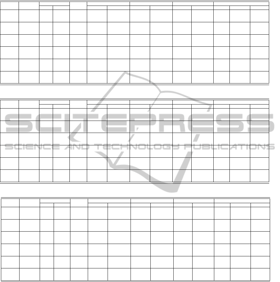
Table 1: Discrete-time model.
Trains Movements Time Before presolve After presolve First solution Number of groups
per group tech. comm. interval Variables Constraints Variables Constraints Solution Solve time solved infeasible no result
Min 5 2 8 77 2140 4624 318 1913 156 0,02
50 0 0Average 5 3 7 77.6 2175 15199 391 7772 155 0.11
Max 5 5 5 51 2140 24684 455 14178 118 1.15
Min 10 3 17 122 4530 28666 754 13457 365 0.08
24 0 0Average 10 7 13 105.7 4598 59962 929 32104 312 2.07
Max 10 9 12 64 4764 89769 1030 49525 254 14.98
Min 15 7 23 94 7170 85283 1429 45439 524 1.15
13 3 0Average 15 10 20 140.3 7268 129144 1604 68617 485 9.80
Max 15 12 18 137 7170 194985 1748 113906 475 64.88
Min 20 13 31 214 11168 150755 2318 74511 815 2.03
8 3 1Average 20 13 27 176.8 10233 215515 2391 112708 650 10.52
Max 20 13 27 140 10060 184949 2300 101232 646 23.59
Min 25 17 33 213 13200 362041 3015 183220 769 9.02
5 1 3Average 25 17 33 220.4 13377 345295 3300 178056 811 19.93
Max 25 21 31 243 13790 265689 3015 142350 902 29.58
Min 30 18 42 188 16590 475438 4348 240245 980 12.36
3 0 5Average 30 23 38 269.0 16800 533594 4490 272449 978 50.97
Max 30 23 39 243 17220 357778 3962 193601 1090 73.88
Table 2: The continuous-time model.
Trains Movements Time Before presolve After presolve First solution Number of groups
per group tech. comm. interval Variables Constraints Variables Constraints Solution Solve time solved infeasible no result
Min 5 2 8 77 2140 4624 318 1913 156 0.02
50 0 0Average 5 3 7 77.6 2175 15199 391 7772 154 0.07
Max 5 5 5 51 2140 24684 455 14178 118 0.50
Min 10 3 17 122 4530 28666 754 13457 300 0.09
24 0 0Average 10 7 13 105.7 4598 59962 929 32104 313 1.03
Max 10 9 12 64 4764 89769 1030 49525 254 5.30
Min 15 7 23 94 7170 85283 1429 45439 528 1.05
13 3 0Average 15 10 20 140.3 7268 129144 1604 68617 487 7.63
Max 15 12 18 137 7170 194985 1748 113906 475 63.45
Min 20 13 31 214 11168 150755 2318 74511 827 1.83
8 4 0Average 20 8 33 176.8 10233 215515 2391 112708 648 7.03
Max 20 13 27 137 10334 151907 2368 79990 617 11.79
Min 25 14 36 149 13494 220090 3184 116923 844 8.92
5 3 1Average 25 14 38 220.4 13377 345295 3300 178056 823 10.61
Max 25 21 31 163 13200 298832 3110 156363 889 15.16
Min 30 18 42 188 16590 475438 4348 240245 992 11.67
3 1 4Average 30 23 38 269.0 16800 533594 4490 272449 973 24.94
Max 30 23 39 376 16590 767565 5160 383502 858 35.24
Table 3: The reduced continuous-time model.
Trains Movements Time Before presolve After presolve First solution Number of groups
per group tech. comm. interval Variables Constraints Variables Constraints Solution Solve time solved infeasible no result
Min 5 2 8 77 2130 2812 304 1013 156 0.00
50 0 0Average 5 3 4 77.6 2165 5651 350 3265 154 0.04
Max 5 5 5 45 2130 18610 422 13545 140 0.20
Min 10 9 11 102 4510 9048 771 6472 256 0.03
24 0 0Average 10 7 13 105.7 4578 18413 753 12649 314 1.71
Max 10 9 12 112 4743 31484 845 23404 254 26.96
Min 15 7 23 94 7140 19883 1100 13133 543 0.94
13 3 0Average 15 10 20 140.3 7238 31139 1164 22499 489 15.13
Max 15 12 18 137 7140 73169 1348 57475 473 166.27
Min 20 13 31 214 11124 30407 1490 18974 841 1.93
8 4 0Average 20 13 27 176.8 10192 42426 1573 30343 657 4.38
Max 20 9 31 163 10020 41532 1560 29595 775 6.30
Min 25 21 31 243 13738 45417 1905 33419 914 4.93
5 1 3Average 25 17 33 220.4 52886 13326 1995 38258 818 10.33
Max 25 11 40 148 13443 44199 2041 30294 832 24.84
Min 30 18 42 188 16530 73634 2386 53136 994 10.20
3 2 3Average 30 23 38 269.0 16739 74726 2407 55610 998 11.43
Max 30 27 33 376 16530 88703 2503 66487 877 12.76
When the value of L is increased, one can find an op-
timal solution but the solving time can also be greatly
increased. For example, setting L = 30 helps to find
solutions to three cases previously labeled infeasible
at the expense of solve time 330 seconds instead of
the average time of 12 seconds. Further experimenta-
tions are necessary so that the value of L is adjusted
in order to get the best tradeoff between the solution
feasibility and the solving time.
5 CONCLUSIONS
This paper describes a mixed-integer linear program
for routing and scheduling trains through a rail-
way station to find a conflict-free schedule, given
the detailed information of commercial movements.
Considering the time representation, we compare
the continuous-time and discrete-time models. The
continuous-time mathematical model satisfies our
computational requirement and decreases the problem
size. Furthermore, to speed up the calculation, we try
AMixed-IntegerLinearProgramforRoutingandSchedulingTrainsthroughaRailwayStation
451

to cut off the redundant constraints and concentrate on
the potential conflicts. Based on the numerical exper-
iments, the improvements of the reduced continuous-
time model are qualified. For the moment, we can
solve example up to 60 trains, 121 movements during
385 minutes. The solve time of the first feasible solu-
tion is 97.8438 seconds. The solve time depends on
the testing example.
To solve problems of larger size, we propose to
use the decomposition methods (Benders, 1962) (Bi-
nato et al., 2001) (Cordeau et al., 1975). All trains are
divided into groups in chronological sequence. The
group solved is considered as the valid constraints of
shared resources for the succedent groups. The adja-
cent groups have common trains as a buffer, i.e. the
group size is 40 and the buffer group size is 20. The
partitioning procedures are followed until the end of
the problem. This method can be used to solve the
real-time train routing and scheduling problem.
REFERENCES
Bai, L., Bourdeaud’huy, T., Castelain, E., and Rabena-
solo, B. (2013). Recherche de plans d’occupation de
voies dans les r
´
eseaux ferroviaires. In 14e conf
´
erence
ROADEF de la soci
´
et
´
e Franc¸aise de Recherche
Op
´
erationnelle et Aide
`
a la D
´
ecision.
Benders, J. (1962). Partitioning procedures for solv-
ing mixed-variables programming problems. In Nu-
merische Mathematik, 4: 238-252.
Binato, S., Pereira, M., and Granville, S. (2001). A new
benders decomposition approach to solve power trans-
mission network design problems. In Numerische
Mathematik, 16(2): 235-240.
Caimi, G. (2009). Algorithmic decision support for train
scheduling in a large railway network. In PhD thesis.
ETH Zurich.
Carey, M. (1994a). Extending a train pathing model from
one-way to two-way track. In Transportation Re-
search B 28 (5): 395-400.
Carey, M. (1994b). A model and strategy for train pathing
with choice of lines, platforms and routes. In Trans-
portation Research B 28 (5): 333-353.
Carey, M. and Carville, S. (2003). Scheduling and platform-
ing trains at busy complex stations. In Transportation
Research A 37 (3): 195-224.
Cordeau, J., Soumis, F., and Desrosiers, J. (1975). A ben-
ders decomposition approach for the locomotive and
car assignment problem. In Transportation Science,
34(2): 133-149.
D’Ariano, A. (2008). Improving real-time train dispatching:
model, algorithms and applications. In PhD thesis. TU
Delft.
D’Ariano, A., Pacciarelli, D., and Pranzo, M. (2007). A
branch and bound algorithm for scheduling trains in
railway network. In European Journal of Operational
Research 183: 643-657.
Floudas, C. and Lin, X. (2004). Continuous-time versus
discrete-time approaches for scheduling of chemical
processes: A review. In Computers and Chemical En-
gineering 28: 2109-2129.
Heller, I. and Tompkins, C. (1956). An extension of a the-
orem of Dantzig’s. In Linear inequalities and related
systems: 247-254. Princeton Univ. Press, Princeton,
NJ.
Hoffman, A. and Kruskal, J. (1956). Integral boundary
points of convex polyhedra. In Linear inequalities
and related systems: 223-246. Princeton Univ. Press,
Princeton, NJ.
Kroon, L., Romeijn, H., and Zwaneveld, P. (1997). Routing
trains through railway stations: Complexity issues. In
European Journal of Operational Research 98: 485-
498.
Kroon, L. and Zwaneveld, P. (1995). Stations: Final re-
port of phase 1, ERASMUS management report series
no.201. In Rotterdam School of Manangement. Eras-
mus University Rotterdam. Rotterdam. Netherlands.
Schrijver, A. and Steenbeek, A. (1994). Dienstregeling on-
twikkeling voor Railned (timetable development for
railway station). In Report Cadans 1.0. C.W.I. Ams-
terdam, Netherlands.
Serafini, P. and Ukovich., W. (1989). Mathematical model
for periodic scheduling problems. In SIAM Journal on
Discrete Mathematics 2: 550-581.
Watson., R. (2001). The effects of railway privatisation on
train planning. In Transport Reviews 21(2): 181-193.
Zwaneveld, P. (1997). Railway planning-routing of trains
and allocation of passenger lines. In PhD thesis. Eras-
mus University Rotterdam. Rotterdam. Netherlands.
Zwaneveld, P., Kroon, L., and Ambergen, H. (1996). A
decision support system for routing trains through
railway stations. In Proceedings of Comp Rail
96:217-226. Computational Mechanics Publications,
Southampton, Berlin.
Zwaneveld, P., Kroon, L., and van Hoesel, S. (2001). Rout-
ing trains through a railway station based on a node
packing model. In European Journal of Operational
Research 128: 14-33.
ICORES2014-InternationalConferenceonOperationsResearchandEnterpriseSystems
452
