
Demand Management for Home Energy Networks using
Cost-optimal Appliance Scheduling
Veselin Rakocevic
1
, Soroush Jahromizadeh
1
, Jorn Klaas Gruber
2
and Milan Prodanovic
2
1
School of Engineering and Mathematical Sciences, City University London, London, U.K.
2
Electrical Systems Unit, IMDEA Energy Institute, Madrid, Spain
Keywords: Smart Homes, Optimization for Efficient Energy Consumption, Energy Profiling and Measurement, Energy
Demand Management, Economic Models of Energy Efficiency.
Abstract: This paper uses problem decomposition to show that optimal dynamic home energy prices can be used to
reduce the cost of supplying energy, while at the same time reducing the cost of energy for the home users.
The paper makes no specific recommendations on the nature of energy pricing, but shows that energy prices
can normally be found that not only result in optimal energy consumption schedules for the energy
provider’s problem and are economically viable for the energy provider, but also reduce total users energy
costs. Following this, the paper presents a heuristic real-time algorithm for demand management using
home appliance scheduling. The presented algorithm ensures users’ privacy by requiring users to only
communicate their aggregate energy consumption schedules to the energy provider at each iteration of the
algorithm. The performance of the algorithm is evaluated using a comprehensive probabilistic user demand
model which is based on real user data from energy provider E.ON. The simulation results show potential
reduction of up to 17% of the mean peak-to-average power estimate, reducing the user daily energy cost for
up to 14%.
1 INTRODUCTION
The emergence of smart homes enables energy
providers to develop sophisticated energy
management solutions, in attempt to optimise energy
production while providing home users with
increased comfort and potential cost reduction. The
future smart homes will be equipped with a range of
control devices and sensing/actuating systems
capable of working together in automatic way to
perform some pre-defined functions. Over the past
decade, the majority of technical challenges for the
home hardware and software solutions have been
solved, and a range of commercial products is
available. For energy providers, the greatest
remaining challenges lie in: (1) development of
intelligent resource management algorithms to
optimise the energy consumption, both at the single-
household level and at the large-scale level; (2)
establishing increased level of trust with the user by
ensuring that the users’ energy consumption data is
kept secret. This paper addresses both of these issues
by providing an optimal distributed algorithm for
home appliance scheduling without the need for
sharing detailed information on daily use of home
appliances.
The process of resource optimisation in home
energy networks has been generating research
interest for several decades now, and in the recent
years it has been accelerated by the technological
advances in sensor networks, smart meters and
actuator systems. In an ideal smart home model, the
historical consumption data, real-time
measurements, pricing, ambient and social aspects
are all used as inputs to optimisation algorithms
which calculate the optimal home appliance energy
consumption schedule. Traditionally, the problem of
optimal use of home energy has been approached in
two ways: (1) reducing consumption, or (2) shifting
consumption. The process of consumption shifting,
also called demand management, or load
management, has been practices by the industry for
several decades, using different forms of load
control (Fahrioglu, 2000, Palensky 2011, Siano
2014). The existing solutions use variable pricing to
generate incentives to home users to shift their
consumption from peak periods, thus reducing the
need to start additional generators, which presents a
21
Rakocevic V., Jahromizadeh S., Gruber J. and Prodanovic M..
Demand Management for Home Energy Networks using Cost-optimal Appliance Scheduling.
DOI: 10.5220/0004854100210030
In Proceedings of the 3rd International Conference on Smart Grids and Green IT Systems (SMARTGREENS-2014), pages 21-30
ISBN: 978-989-758-025-3
Copyright
c
2014 SCITEPRESS (Science and Technology Publications, Lda.)

major cost factor for energy providers.
There is a number of research works that take on
this challenge, and develop algorithms and network
protocols for optimal demand management. For
example, Li, Chen and Low (Li, 2011) show that
there exist time-varying prices that can align
individual optimality with social optimality. In their
model, the utility company collects forecasts of total
demands from all customers, and then sets the prices
to the marginal cost. Each customer updates its
demand and charging schedule. Similarly, Pedrasa,
Spooner and MacGill (Pedrasa, 2010) present a
solution which enables end-users to assign values to
desired energy services, and then schedule the
resources to maximise the users’ benefits. They
propose the use of particle swarm optimisation,
because of simple implementation. They do not,
however, test their solution on large-scale systems
and do not prove the optimality of the solution.
Zakariazadeh, Jadid and Siano (Zakariazadeh, 2014)
propose a multi-objective framework, based on
augmented ε-constraint method, to minimize the
total operational costs and emissions and to generate
Pareto-optimal solutions for the energy and reserve
scheduling problem. In the work of Ramchurn et al
(Ramchurn, 2011, Vytelingum, 2010) decentralised
demand side management is realised through the
process of cooperation between the smart meters
(‘agents’). The meters receive the costs of
generating electricity to the consumers, and use
learning mechanisms to gradually adapt the agents’
deferrable energy load based on the predicted market
prices for the next day. Similar approach is also
taken by (Mohsenian-Rad, 2010), (Ganu, 2012), and
(Ibars, 2010) . In these solutions the end-users are
somehow made to voluntarily adjust their
consumption. (Mohsenian-Rad, 2010) formulates an
energy consumption scheduling game, where the
players are the users and their strategies are the daily
schedules of their household appliances and loads.
Similarly, (Ibars, 2010) bases the solution on a
network congestion game, which can be
demonstrated to converge in a finite number of steps
to a pure Nash equilibrium solution. (Jain, 2013)
goes one step further, by applying the concept of
bargaining / auctioning of energy resources on the
smart grid including electric vehicles.
It is important to stress that most of these works,
including ours, rely on consumer’s willingness to
act. In other words, the end-user benefit is always
modelled through cost, and optimality of the
scheduling is based on the process of cost
minimisation. The mechanism of costing allows the
users to react, in their own interest. Dynamic pricing
and its drawbacks are analysed in great detail in the
past research, e.g. in (Borenstein, 2002) and
(Roozbehani, 2010). In a response to this, (Wijaya,
2013) proposes an interesting approach to cut the
peak to average energy ratio explicitly from the
supply side. The resulting load cuts are then
distributed among consumers by the means of a
multiunit auction which is done by an intelligent
agent on behalf of the consumer.
In this paper, we decompose the provider and the
user optimization problem to prove that, if energy
prices are set as optimal consistency prices, the
energy provider’s revenue at optimal energy
consumption levels is greater than the variable cost
of supplying energy. This motivates the design of a
heuristic real-time algorithm where at every timeslot
each appliance energy consumption is updated
according to the real-time energy price and
estimated price of operating each appliance. The
home can then use this to calculate the optimal
energy consumption schedule. The paper makes no
specific recommendations on the nature of energy
pricing, but shows that energy prices can normally
be found that not only result in optimal energy
consumption schedules for the energy provider’s
problem and are economically viable for the energy
provider, but also reduce total users energy costs.
The paper shows that optimal dynamic energy prices
can be used to pass on the reduction in the cost of
supplying energy to the users, when sufficiently
scaled down. This provides financial incentives to
users to subscribe to the smart home scheme. The
presented algorithm ensures users’ privacy by
requiring users to only communicate their aggregate
energy consumption schedules to the energy
provider at each iteration of algorithm.
To evaluate the performance of the optimisation
algorithm, we use a comprehensive consumer
demand model to compute the quantitative benefits
of the algorithm. The model is described in section
4; it is based on appliance definition, user profile
generation and daily appliance use determination,
and is based on real user data from energy provider
E.ON and the UK Government Report on home
energy use (Zimmermann, 2012). The performance
evaluation of the new algorithms is done using
simulation, the details of which are given in section
5.
The simulation results show that applying the
new optimisation algorithm, it is possible to reduce
the mean power peak to average ratio (PAR)
between 0.16 and 0.35 with 99% probability. That is
between 7.83% and 17.02% of the original time
series mean PAR estimate. Furthermore,
SMARTGREENS2014-3rdInternationalConferenceonSmartGridsandGreenITSystems
22

optimisation reduces average user daily energy cost
between 3.54% and 14.72% of its original time
series mean estimate with 99% probability.
It is worth noting that reading and understanding
the simulation results for the large-scale home
energy networks is very difficult, as averaging the
benefits of optimal energy supply gives only a part
of the full picture. It is for this reason that we
believe that the best practical use of the research
results presented in this paper is to integrate them in
the development of energy consumption
visualisation tools for the individual users and for
the energy supplier. Visualisation of energy
consumption (Goodwin, 2013) will enable better
understanding of the pattern of energy use and the
consequence of optimisation and optimal appliance
schedules.
2 SYSTEM MODEL
We start by presenting a model for energy users and
energy provider. The user is modeled as an operator
of a set of home appliances which operate over a
finite scheduling time horizon. The user’s objective
is to choose feasible energy consumption schedule
so as to minimize the cost of energy. The provider,
on the other hand, benefits from selling units of
energy to the users. Critically, the objective of the
provider is to minimize the cost of supplying the
energy consumed by the users by shifting the total
energy consumed during the time horizon.
We consider a smart power network comprising
a set of users served by an energy provider who
participates in the wholesale energy market. Each
user is equipped with a smart meter capable of
scheduling energy consumption of appliances, and
smart meters are connected to the energy provider
via a communication link. In the following sections,
we describe how users and the energy provider are
modeled.
Users: We assume each user ∈ operates a set of
appliances including photovoltaic (PV)
appliances, which are operated over a finite
scheduling time horizon (e.g. a day) divided into
timeslots (e.g. 15 minutes). We denote by the set
of timeslots in the scheduling time horizon. For each
user ∈, we denote by
,
the energy
consumption scheduled for appliance ∈
at time
∈, where negative values of
,
represent power
generation. Let
,
≜
,
,∈be the energy
consumption schedule vector for appliance∈
,
and
≜
,
,∈
be the energy consumption
schedules for all appliances. We also denote the
cardinality of sets by capital letters, e.g. N
|
|
and T
|
|
. We assume that each appliance∈
requires a total energy of
,
during the scheduling
horizon, i.e.
,
,
∀∈
∈
(1)
In addition, we assume that each appliance∈
can use a minimum power level of
,
,
and a
maximum power level of
,
,
at timeslot ∈ , i.e.
,
,
,
,
,
∀∈,∈
(2)
Clearly, if appliance∈
is non-controllable
then
,
,
,
,
≜
,
, ∀∈ and
∑
,
∈
,
.
User Optimisation Problem: Let
be the unit price
of energy at time ∈, which is set by the energy
provider. We assume that users cannot sell their
excess generated energy to the energy provider.
Given the energy price vector
,∈
, the
objective of user ∈ is to then choose feasible
energy consumption schedules
so as to minimize
total energy costs, i.e. to solve the following
optimization problem:
min
max
,
,0
∈
∈
s.t. (1) and (2)
(3)
Evidently, optimal solution of (3) is dependent on
the energy prices set by the energy provider.
Energy Provider: The energy provider is
characterized by its energy cost function and its
optimization objectives. The cost function
represents the cost for the energy provider to supply
0units of energy at time ∈ and is widely
assumed to be increasing and strictly convex (see
e.g. (Li, 2011) and (Mohsenian-Rad, 2010) As an
example, the energy cost function for thermal
generators is shown to be quadratic as follows
(Mohsenian-Rad, 2010):
∈
(4)
where
,
0 and
0.
Optimisation Objectives: Since by constraint (1)
users’ energy demands during the scheduling
horizon are fixed, we define the energy provider’s
objective as to minimize the cost of supplying the
energy consumed by the users by shifting the total
energy consumption at each time slot, i.e. to solve
the following optimization problem
N
DemandManagementforHomeEnergyNetworksusingCost-optimalApplianceScheduling
23

min
,
,0
∈
∈
∈
s.t. (1) and (2) ∈
(5)
where
,∈
. The optimization problem
(5) is convex and can be solved by the energy
provider in a centralized fashion, providing that
users energy demand constraints are available to the
energy provider. Alternatively, (5) can be solved
jointly by the energy provider and users using a
distributed algorithm. In either way, appropriate
energy pricing schemes have to be designed to
ensure user participation by providing financial
incentives.
3 OPTIMISATION ALGORITHM
Since the objective function in the energy provider’s
optimisation problem (5) is not strictly convex in x,
computation of primal optimal solutions from the
dual optimal solutions may not be possible (Boyd,
2004). As here we adopt a dual decomposition
approach, we use the generalization of proximal
minimization algorithm proposed by (Lin, 2006) that
can be applied to the problems with similar form as
(5). First, using the auxiliary vector ≜
,∈
, where
≜
,
,∈
,
,
≜
,
,∈
, we transform the optimization problem (5) into
the following equivalent form
,
,
∈
∈
1
2
,
,
∈
∈
∈
s.t. (1) and (2) ∈
(6)
where
0∈. Let x
*
be the optimal solution
of (5). Then
∗
and
∗
is the optimal
solution of (6). The optimization problem (6) can
then be solved using the algorithm as presented in
(Lin, 2006):
Algorithm A: Fix K1. At iteration:
1. Fix zz
j
and estimate the solution of
the dual problem of (6) by applying
gradient method on dual variable for
iterations.
2. Let
1,0
,
. Let be the
primal variable associated with the dual
variable
,
. Set
,
1
,
,
,
∀∈,∈
,∈,
where 0
1,∀∈ .
(7)
We now focus on development of a distributed
algorithm for step 1 of algorithm A at iteration.
Note that optimization problem (6) is strictly convex
when z is fixed. Introducing the auxiliary variable
,
∈
∈
∀∈
(8)
The optimization problem becomes
,
1
2
,
,
∈
∈
∈
s.t. (1), (2) ∀∈ and (8)
(9)
The Lagrangian after relaxation of constraint (8)
is (ρ,y,x)
∑
∑∑
,
∈
∈∈
,
∑∑
,
∈
∈
, where is
the vector of consistency prices. The dual problem is
then
max
(10)
where
min
,
,,
,
s.t. (1) and (2) ∀∈
(11)
Since (9) is strictly convex, the dual function
(11) is differentiable and its gradient is given by
(Bertsekas, 1999):
,
∈
∈
∀∈
(12)
where
,
is the solution of (11) given
,
. The dual problem (10) can then be solved
using gradient method as follows
,1
,
,
,
,
∈
∈
,∀
∈
(13)
where
,
,
,
denote the solution of (11)
given
,
. Let the primal-dual pair
∗
,
∗
denote the stationary point of algorithm A defined
by
∗
argmax
∗
,
∗
,
∗
,
s.t. (1), (2) ∀∈
∗
,
,∗
∈
∈
∀∈
By KKT optimality conditions (Boyd, 2004) for
any stationary point
∗
,
∗
∗
is the optimal
solution of (6). It is shown in (Lin, 2006) that when
in (13) is small enough, algorithm A converges to
SMARTGREENS2014-3rdInternationalConferenceonSmartGridsandGreenITSystems
24

a stationary point
∗
,
∗
.
The dual function
can be decomposed into
two subproblems
, where
min
∈
(14)
and
min
∑∑∑
,
∈
∈∈
,
,
, s.t. (1), (2) ∀∈
(15)
Subproblem (6) is an unconstrained convex
minimisation problem and due to the strict convexity
of
,∈, has a unique solution. Let
be the
unique solution of (14). Then
∀∈
(16)
Thus
∀∈
(17)
Equation (17) can be computed by the energy
provider for each timeslot ∈independently,
given the associated consistency price
.Subproblem (15) can be decomposed into
optimisation problems for individual users:
∑
,∈
, where
,
min
∑∑
,
∈
∈
,
,
s.t. (1), (2)
(18)
It can be noted that at the stationary point of
algorithm A the quadratic term in the objective
function of (18) is zero and (18) is equivalent to the
user optimization problem (3) with
∗
.Hence,
optimal consistency prices can be interpreted as
energy prices that encourage users to opt for optimal
energy consumption schedules for the energy
provider’s problem (5), in order to minimise their
energy costs under these prices. We will show later
in the next section that reduction in the cost of
energy supply as a result of solving (5) can be
passed on to the users, if energy prices are based
on adequately scaled down optimal consistency
prices
∗
.
The user optimization problem (18) can be
further decomposed into optimisation problems for
individual appliances as
,
∑
,,
∈
, where
,,
min
,
∑
,
∈
1
2
,
,
2
s.t. (1), (2)
(19)
Using dual decomposition, (19) can be
decoupled into appliance optimization problem for
each time slot. The Lagrangian after relaxation of
constraint (1) is
,
,
,
,
1
2
,
,
∈
,
,
,
∈
,
where
,
is the Lagrange variable associated with
constraint (1) or price of operating appliance ∈
. The dual problem is then
max
,
,,
,
(20)
where
,,
,
min
,
,
,x
,
s.t. (2)
(21)
The dual function (21) can be decoupled into
appliance optimization problems for each time slot:
,,
,
∑
,,
∈
,
,
,
,
where
,,
,
min
,
,
,
,
,
s.t.(2)
(22)
Let
,
,
be the solution of (22). Then
,
,
,
,
,
,
,
,
(23)
We consider two measures of performance,
namely, peak- to-average ratio (PAR) and average
user daily energy cost, to evaluate the benefits of
optimization to the energy provider and users,
respectively. PAR is defined as the ratio of daily
peak to average load, and used here as a measure of
variation of aggregate daily energy consumption. It
is defined by
max
∈
∑∑
,
∈
∈
∑∑
,∈
∈
(24)
The average user daily energy cost is defined as
the daily cost of supplying energy divided by the
number of users, and used to measure the minimum
possible daily energy cost that can be passed on to a
user on average:
∑
∑
max
∑
,
,0
∈
∈
∈
(25)
Considering this solution, the proposed approach
for solving the energy provider’s optimization
problem (5) can then be summarized as the
following distributed algorithm:
Algorithm A: Fix 1. At
iteration:
1. Fix
and run algorithm S for K
DemandManagementforHomeEnergyNetworksusingCost-optimalApplianceScheduling
25

iterations.
2. Let
1,0
,
. Let
be the
primal variable associated with the dual
variable
,
. Set
,
1
,
,
,
∀∈
,
,∈
,∈
(26)
Where 0
1,∀∈.
Algorithm S: At
iteration:
1. Given the consistency prices
,
, each
user ∈
computes:
the price of operating each appliance
,
,
, ∈
, by solving (20)
appliance energy consumption schedule
,
,
, ∈
, ∈
,
, using (23), and
communicates its aggregate energy
consumption schedule
∑
,
,
∈
,
∈
,
, to the energy provider.
2. Given the consistency prices
,
, the
energy provider computes:
the auxiliary variable
,
, ∈
, using
(17),
updates the consistency price
,
,
given the aggregate energy
consumption schedules for all users
∑∑
,
,
∈
∈
and
,
, ∈,
according to the gradient algorithm (13).
Note that the proposed algorithm ensures users’
privacy by requiring users to only communicate their
aggregate energy consumption schedules to the
energy provider at every iteration of algorithm S.
Note also that, with the exception of computation of
,
,
, ∈
, all the computations can be
further decoupled across individual timeslots. This
motivates the heuristic real-time algorithm presented
in the following sections where at every timeslot
each appliance energy consumption is updated
according to the real-time energy price and
estimated price of operating each appliance
,
,
, ∈
.
As discussed in the previous section, optimal
energy consumption schedules for the energy
provider’s problem (5) can be attained if energy
prices are set as optimal consistency prices
∗
, i.e.
setting
∗
, energy consumption schedules that
are minimizers of the users optimization problem (3)
are also minimizers of the energy provider’s
problem (5). Moreover, as stated in the following
theorem, the energy provider’s revenue based on
energy prices
∗
is greater than the variable cost of
supplying energy, at optimal energy consumption
levels.
Theorem 1. If energy prices are set as optimal
consistency prices
∗
, the energy provider’s revenue
at optimal energy consumption levels is greater than
the variable cost of supplying energy, i.e.
∗
∗
∗
0
,∀∈
(27)
Proof. Since we assumed that
is increasing and
strictly convex, it follows from the first order
condition for strict convexity (Boyd, 2004) that
∗
∗
∗
0
∀∈
(28)
replacing (16) in the above inequality then yields
(27).
However, we are interested in energy pricing
scheme that not only results in optimal energy
consumption schedules for the energy provider’s
problem (5) and covers the variable cost of
supplying energy, but also reduces or ideally
minimizes users energy costs, in order to ensure
users participation in the smart home scheme.
To examine the existence of such scheme note
that by the mean value theorem (Bertsekas, 1999)
there exists
∈0,
∗
for all ∈ such that
∗
∗
0
∀∈
(29)
It follows from (28) that there exists 0 < t < 1,
for all ∈ , such that
∗
∀∈
(30)
Let
∈
. Then,
∗
∗
∀∈
(31)
So,
∗
∗
∈
∗
∗
∈
∗
∈
∗
0
∈
(32)
The term on the right side of the above equality
is the minimum daily cost of supplying energy and
hence is the lower bound on the viable total users
energy costs at optimal energy consumption levels.
Note that users optimization problem (3) with
energy prices
∗
is equivalent to the case
when
∗
and thus result in optimal energy
consumption schedules for the energy provider’s
problem (5). The above inequality states that there
exist energy prices that lead to optimal energy
consumption schedules for the energy provider’s
problem (5), economically viable for the energy
provider and result in lower viable total users energy
SMARTGREENS2014-3rdInternationalConferenceonSmartGridsandGreenITSystems
26
costs than with energy prices
∗
, but not necessarily
the minimum viable level. This implies that, unless
the current energy consumption schedules are very
close the levels that optimize the energy provider’s
problem (5), energy prices can normally be found
that not only result in optimal energy consumption
schedules for the energy provider’s problem (5) and
are economically viable for the energy provider, but
also reduce total users energy costs. In the case of
quadratic cost function (4), it follows from (29) that
∗
, ∈ . If 0in (4), then
, for all ∈ . Thus, in this case energy prices
∗
results in minimum total users energy costs
at optimal energy consumption levels, while still
economically viable for the energy provider.
Notice that if the objective function in the energy
provider’s problem (5) is scaled by a positive
constant 0, the resulting optimization problem
is equivalent to (5) and hence the minimum cost of
supplying energy, and by (16), optimal consistency
prices
∗
are also scaled by 0.
4 CONSUMER DEMAND MODEL
To evaluate the algorithm performance in detail, it is
necessary to use a comprehensive household
consumer energy demand model. The model –
developed specifically for this project - generates
artificial consumption data, both for a single
household and an entire neighbourhood. The model
has been developed on the basis of real home user
data generated at the E.ON testbed facility in the UK
in 2012.
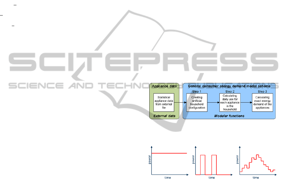
The model generates the consumption data of the
households in the following three main steps (Figure
1): (1) determining the household configuration (i.e.
which appliances can be found in a household); (2)
computing the daily use of each appliance (i.e. how
many times is an appliance used on a certain day);
(3) calculating the exact energy demand of each
appliance (i.e. at what time is the appliance used on
a certain day)
The different steps of the consumer energy
demand model are based on probabilistic approaches
using basic appliance definitions for the generation
of the consumption data. The general model
structure uses some basic appliance definitions to
generate the synthetic consumption data in three
main steps: (1) Basic appliance definition; (2) User
profile generation; (3) Daily appliance use
determination.
The most common household appliances can be
classified according to a reduced number of
simplified power level patterns (Yao, 2012,
Richardson, 2010, Carpaneto, 2007). In the proposed
model three different power level patterns for the
approximation of the demand curve have been
considered (Figure 2). Pattern 1 represents
continuously running appliances with a constant
power level, such as fridges or freezers. Pattern 2
allows the approximation of occasionally operated
appliances with possible non-zero energy
consumption in standby operation such as washing
machines or TVs. Finally, pattern 3 is used to
approximate the power curve.
The three simplified power level patterns were
used in the development of a classification scheme
based on different usage types. These usage types
take into account factors such as frequency, duration
and time of use of the considered appliances and
allow a classification closely related to the customer
habits.
Figure 1: General structure of the developed consumer
energy demand model.
Figure 2: Classification of household appliances by power
level patterns.
The consumer energy demand model determines
in the first step the configuration of one or several
households. For most appliance types, the number of
devices is computed using a probabilistic approach.
However, exceptions have been considered for a few
appliances. The computation of the number of
devices of a certain appliance type is based on a
binomial distribution in order to obtain certain
variation around a desired average value.
Finally, an important aspect of the model is
consideration of exceptions. In our case, special care
was taken: (1) to accurately represent lighting, (2) to
exclude appliances which exist with gas and
electricity connections; (3) to limit the sum of
electric and gas space heaters to one device per
DemandManagementforHomeEnergyNetworksusingCost-optimalApplianceScheduling
27
household (This limitation is also used in the case of
water heating appliances). For a detailed description
of the developed usage types and a complete list of
the considered appliances the reader is referred to
(Gruber, 2012).
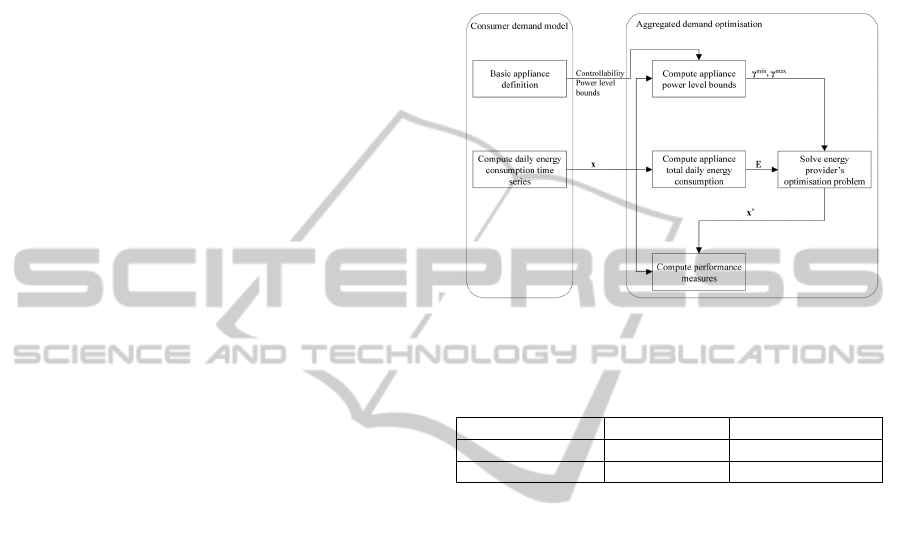
The household consumer energy demand model
is used in the remainder of the paper to simulate the
representative households in order to evaluate the
performance of the optimal algorithms presented in
section 3. Figure 3 shows the link between
consumer demand model and aggregated demand
optimisation algorithm, at each simulation
replication. The appliance total daily energy
requirements E≜
,
,∈
,∈ is computed
from the daily energy consumption time series x
generated by the proposed consumer demand model.
5 IMPLEMENTATION AND
SIMULATION RESULTS
Having defined the model and the theoretical
optimisation algorithm in the previous sections, in
this section we focus on the actual implementation
of the algorithm.
Using the controllability and power level data
from the basic appliance definition, minimum and
maximum power levels
≜
,
,
,∈
,∈
,∈ and,
≜
,
,
,∈
,∈,∈
are set equal to the energy consumption time
series for non-controllable appliances, and to the
minimum and maximum power level for fully
controllable appliances. Here, we refer to appliances
with no operational timing constraints as fully
controllable appliances. For partially controllable
appliances the values of these parameters are set
according to their specific constraints, as will be
explained later in the simulation results. Given the
values of parameters ,
,
, the optimal
energy consumption schedules
∗
are computed
using the algorithm described in Section 3. Finally,
daily estimates of mean performance measures are
computed for the original energy consumption time
series and its optimisation, given the values of x and
∗
, respectively.
The simulation experiment involved generation
of energy consumption time series and its
optimization for 100 users for 12 independent weeks
during a typical winter season. For each week,
energy consumption time series and its optimized
version were generated separately for every
weekday with sampling time of 15 minutes. The
Peak to Average Ratio (PAR) and the average user
daily energy cost were subsequently measured for
each weekday and used to estimate their mean
values for the week. In the optimisation model, the
operation time of washing appliances were assumed
to be flexible throughout the day and hence treated
as a control variable.
Figure 3: Interface between consumer demand model and
aggregated demand optimization results.
Table 1: PAR Values.
PAR values weekday weekend
original 2.16 1.78
optimised 2.05 1.65
Furthermore, the power level of heating and cold
appliances were assumed to be adjustable within the
range of 10% of their original time series values and
treated as additional control variables. The daily
energy requirement of these types of appliances was
assumed to be fixed and equal to their daily usage
generated by the consumer demand model. Power
levels and operation times of the remaining
appliances were set equal to their original time series
values. The energy cost function was assumed to be
of the form (4) with parameters
0.1,
0,
0, for all ∈.
The simulation results indicate that the original
time series peak loads during the late afternoon/early
night at weekday are significantly higher than
weekend as indicated by their respective PAR values
of 2.16 and 1.78. In these examples, optimisation
reduces the load variation resulting in PAR values of
2.05 and 1.65 for the example weekday and
weekend, respectively (Table 1).
Figure 4 shows the resulting aggregate energy
consumption time series and its optimisation for a
typical weekday (similar results for weekend exist,
the figure is omitted because of the space
constraints). Figure 5 gives a better visualization of
the benefit of optimization, using the load duration
SMARTGREENS2014-3rdInternationalConferenceonSmartGridsandGreenITSystems
28
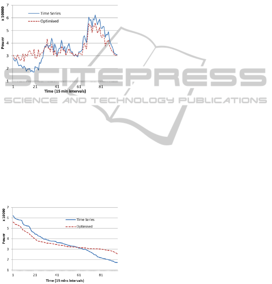
curve to show the gains made in the peak demand
using out optimization algorithm. The load duration
curve shows the energy consumption data by 15-
minute intervals, sorted in descending order. Results
presented in Figures 4 and 5 show average values for
100 households, with individual household gains
greatly depending on the household model.
Figure 4: Aggregate energy consumption time series and
its optimisation for 100 users for a typical weekday.
The overall simulation results indicate that
optimisation reduces mean PAR between 0.16 and
0.35 with 99% probability. That is between 7.83%
and 17.02% of the original time series mean PAR
estimate. Notice that this is despite the fact that the
optimisation objective was to minimise the quadratic
energy cost function, rather than to minimise the
PAR explicitly. Furthermore, optimisation reduces
average user daily energy cost between 3.54% and
14.72% of its original time series mean estimate
with 99% probability, for all γ>0 multiples of
parameters
,∈.
Figure 5: Load Duration Curve for aggregate energy
consumption for 100 users on a typical weekday.
As it was mentioned in the Introduction section,
averaging the benefits of optimal energy supply
rarely gives the full picture. The optimisation
presented in this paper can be used in the design and
development of user visualisation tools. These tools
can be used by home users to understand better the
benefits of optimal appliance schedule at their home.
For more details about the potential use of data
visualisation in energy networks the reader is
referred to (Goodwin, 2013).
6 CONCLUSIONS
This paper looks into the problem of optimal use of
energy in homes. The paper uses problem
decomposition to show that optimal dynamic home
energy prices can be used to reduce the cost of
supplying energy, while at the same time reducing
the cost of energy for the home users. We provide a
proof that if energy prices are set as optimal
consistency prices, the energy provider’s revenue at
optimal energy consumption levels is greater than
the variable cost of supplying energy. This is then
used to design a heuristic real-time algorithm for
demand management using home appliance
scheduling. The performance of the algorithm is
evaluated using simulation, where a comprehensive
model of home energy consumption is used.
In terms of the future work, the focus will be on
two issues: (1) the detailed performance evaluation
of the presented algorithm, using concrete pricing
idea, a larger variety of objective functions,
including peak minimisation and optimisation of
user comfort/discomfort, and realistic models of user
reaction; (2) utilising the linear time complexity
(O(n)) of our algorithm, which makes it suitable for
performing simulation on very large sets of data
(entire city or country) using cluster/cloud
computing in a very short time for interactive energy
data analysis and visualisation. In our future work,
we will aim to experiment with the efficiency of the
algorithm for large-scale optimisation and
visualisation of household energy use, to understand
better the nature of the energy price from the user
point of view.
ACKNOWLEDGEMENTS
The authors would like to thank E.ON International
Research Initiative for providing support for this
work. Also, we would like to thank Sara Jones,
Jason Dykes, and their teams from the School of
Informatics, City University London, for their
cooperation on the project.
DemandManagementforHomeEnergyNetworksusingCost-optimalApplianceScheduling
29

REFERENCES
Fahrioglu M. and Alvardo F. L., 2000, “Designing
incentive compatible contracts for effective demand
managements,” IEEE Trans. Power Systems, vol. 15,
no. 4, pp. 1255–1260.
Palensky P., Dietrich D., 2011, Demand Side
Management: Demand Response, Intelligent Energy
Systems, and Smart Loads, IEEE Transactions on
Industrial Informatics, 7(3).
Siano P., 2014, Demand response and smart grids - A
survey, Renewable and Sustainable Energy Reviews,
30, pp 461-478.
Li N., Chen L., and Low S. H., 2011, Optimal demand
response based on utility maximization in power
networks. In Proceedings of IEEE Power and Energy
Society General Meeting.
Pedrasa M., Spooner T., MacGill I., 2010, Coordinated
Scheduling of Residential Distributed Energy
Resources to Optimise Smart Home Energy Services,
IEEE Transactions on Smart Grid, 1(2).
Zakariazadeh A., Jadid S., Siano A., 2014, Economic-
environmental energy and reserve scheduling of smart
distribution systems: A multiobjective mathematical
programming approach, Energy Conversion and
Management, 78, pp. 151-164.
Ramchurn S., Vytelingum P., Rogers A., Jennings N,
2011, Agent-based Control for Decentralised Demand
Side Management in the Smart Grid, Proc. Of 10th
International Conference on Autonomous Agents and
Multiagent Systems – Innovative Applications Track
(AA-MAS 2011), May 2011, Taiwan.
Vytelingum P., Voice T. D., Ramchurn S. D., Rogers A.,
Jennings N R, 2010, Agent-based micro-storage
management for the smart grid, In Proc. Of the 8th
Conf Autonomous Agents and Multiagent Systems
AAMAS 2010, pages 39-46,
Mohsenian-Rad A., Wong V. W.S., Jatskevich J., Schober
R., and Leon-Garcia A.. 2010, Autonomous demand-
side management based on game-theoretic energy
consumption scheduling for the future smart grid.
IEEE Transactions on Smart Grid, 1(3):320–331.
Ganu T., Seetharam D. P., Arya V., Kunnath R., Hazra J.,
Husain S. A., De Silva L. C., and Kalyanaraman S.,
2012, “nplug: a smart plug for alleviating peak loads,”
in Proceedings of the 3rd International Conference on
Future Energy Systems: Where Energy, Computing
and Communication Meet, ser. e-Energy ’12. New
York, NY, USA: ACM, pp. 30:1– 30:10.
Ibars C., Navarro M. Giupponi L., 2010, Distributed
Demand Management in Smart Grid with a
Congestion Game, Smart Grid Communications
(SmartGridComm), First IEEE International
Conference on.
Jain S., Narayanaswamy, Narahari Y., Hussain S. A.,
Yoong V. N., 2013, Constrained Tâtonnement for Fast
and Incentive Compatible Distributed Demand
Management in Smart Grids, e-Energy’13.
Wijaya T. K., Larson K., Aberer K., 2013, Matching
Demand with Supply in the Smart Grid using Agent-
Based Multiunit Auction, Communication Systems and
Networks (COMSNETS), Fifth International
Conference on.
Borenstein S., Jaske M., Rosenfeld A. 2002, Dynamic
pricing, advanced metering, and demand response in
electricity markets. UC Berkeley: Center for the Study
of Energy Markets,
Roozbehani M., Dahleh M., Mitter S., 2010 Dynamic
Pricing and Stabilization of Supply and Demand in
Modern Electric Power Grids, Smart Grid
Communications (SmartGridComm), First IEEE
International Conference On.. 543-548.
Zimmermann J.-P., Evans M., Griggs J., King N., Harding
L., Roberts P., Evans C. 2012, Household Electricity
Survey: A study of domestic electrical product usage,
Tech. rep., Department for Environment, Food and
Rural Affairs - Department of Energy and Climate
Change - Energy Saving Trust.
Boyd S. and Vandenberghe L., 2004. Convex
Optimization. Cambridge University Press,
Cambridge, UK,
Lin X. and Shroff N. B.. 2006, Utility maximization for
communication networks with multipath routing. IEEE
Transactions on Automatic Control, 51(5):766–781.
Bertsekas D. P. 1999. Nonlinear Programming. Athena
Scientific, Belmont, Massachusetts.
Gruber J., Prodanovic M. 2012, Residential Energy Load
Profile Generation Using a Probabilistic Approach, in:
Proceedings of the 2012 Sixth UK Sim/AMSS
European Symposium on Computer Modeling and
Simulation (EMS), pp. 317 –322.
Yao R. and Steemers K. 2012, A method of formulating
energy load profile for domestic buildings in the UK,
Energy and Buildings, 37(6), pp. 663–671.
Richardson I., Thomson M., Infield D., and Clifford C.,
2010, Domestic electricity use: A high-resolution
energy demand model, Energy and Buildings, vol. 42,
no. 10, pp. 1878–1887.
Carpaneto E. and Chicco G., 2007, Probabilistic
characterisation of the aggregated residential load
patterns, IET Generation, Transmission &
Distribution, 2(3), pp. 373–382.
Goodwin, S, Dykes, J., Jones, S., Dillingham, I., Dove, G.,
Duffy, A., Kachkaev, A., Slingsby, A., Wood, J. 2013,
Creative user-centered visualization design for energy
analysts and modelers. IEEE transactions on
visualization and computer graphics (1077-2626), 19
(12), p. 2516.
SMARTGREENS2014-3rdInternationalConferenceonSmartGridsandGreenITSystems
30
