Online Knapsack Problem with Items Delay

Hajer Ben-Romdhane

and Saoussen Krichen

1,2

LARODEC Laboratory, ISG of Tunis, 41 Rue de la Libert´e, Le Bardo, Tunisia

FSJEG de Jendouba, Avenue de l’U.M.A, 8189 Jendouba, Tunisia

Keywords:

Online Optimization, Dynamic Programming, Knapsack problems, Optimal Stopping Problems.

Abstract:

We address in this paper a special case of the online knapsack problem (OKP) that considers a number of

items arriving sequentially over time without any prior information about their features. As items features are

not known in advance but revealed at their arrival, we allow the decision maker to delay his decision about

incoming items (to select the current item or reject it) until observing the next ones. The main objective

in this problem is to load the best subset of items that maximizes the expected value of the total reward

without exceeding the knapsack capacity. The selection process can be stopped before observing all items

if the capacity constraint is exhausted. To solve this problem, we propose an exact solution approach that

decomposes the original problem dynamically and incorporates a stopping rule in order to decide whether to

load or not each new incoming item. We illustrate the proposed approach by numerical experimentations and

compare the obtained results for different utility functions using performance measures. We discuss thereafter

the effect of the decision maker’s utility function and his readiness to take risks over the ﬁnal solution.

1 INTRODUCTION

Online optimization problems model a large range of

real-world situations where the problem inputs are

revealed over time (Mahdian et al., 2012). In such

problems, the ﬁnal decision is made up of many sub-

choices that are taken before all data become avail-

able. For instance, in the problem of hiring em-

ployees, candidates applying for the position arrive

sequentially and are interviewed one by one. The

employer is required to make an irrevocable deci-

sion about each interviewed candidate before receiv-

ing the next ones, and while knowing nothing about

their competency. Practical applications of online

optimization problems arise in (but not limited to):

dynamic resource allocation, inventory management,

machine scheduling, and auctions. These problems

require algorithms that make the decision in an online

fashion for many considerations, among which: the

importance of real-time decision making (e.g., many

requests may become unavailable after some time, the

value of a given offer may decrease by time, or ad-

ditional costs may be incurred), and waiting that all

data become available is costly (in terms of time and

in terms of loss of good opportunities). An “online al-

gorithm” is an algorithm that must make the decision

sequentially over time based only on the previously

served requests and with partial or imperfect knowl-

edge about the potential ones (Albers, 2003).

In this article, we are particularly concerned with

the knapsack problem (KP), one of the most widely

and extensively studied combinatorial optimization

problems that knew several variations and extensions

over years. In its static version (0-1KP), we are given

a number of items from which we are required to se-

lect a subset to be carried into a knapsack of a lim-

ited capacity. Items differ from each other by their

rewards and their weights. The problem is to load

the subset of items which maximizes the total reward

of the knapsack contents without exceeding its ca-

pacity. This variant of the KP supposes the simul-

taneous availability of all items as well as a com-

plete knowledge about their features (weight and re-

ward). However, many real-world applications of

the KP involve receiving items in an online man-

ner (Kleywegt and Papastavrou, 1998)(Babaioffet al.,

2007). This includes web advertising, selling real-

estate, and auctions (Zhou et al., 2008). Accordingly,

the online knapsack problem (OKP) was introduced

in (Marchetti-Spaccamela and Vercellis, 1995), and

investigated since then in several studies. In (Iwama

and Taketomi, 2002), it was shown that the OKP is

inapproximable and that a relaxation (e.g. to assume

that items are removable, or to allow resource aug-

213

Ben-Romdhane H. and Krichen S..

Online Knapsack Problem with Items Delay.

DOI: 10.5220/0004832702130220

In Proceedings of the 3rd International Conference on Operations Research and Enterprise Systems (ICORES-2014), pages 213-220

ISBN: 978-989-758-017-8

 2014 SCITEPRESS (Science and Technology Publications, Lda.)

mentation) is needed to approach the optimal solution

within a constant ratio.

This work introduces a new relaxed version of the

OKP that allows the delay of arriving items. We de-

ﬁne the delay of an item as being the defer of the de-

cision about that item until observing the next one(s).

That is, an item i received at t will still available for

the selection in subsequent stages until it is loaded in

the knapsack (at any stage g >= t) or the decision pro-

cess ends (when all the potential items are received).

Indeed, the OKP with delay is a more fair model of

many real world scenarios where the revealed offers

still available until a given deadline after which they

are loosened. Therefore, discarding these offers early

from the selection process may proveregrettable if the

subsequent offers are less desirable. We note that the

delay of offers in online optimization problems has

been considered previously in the literature, namely

with the optimal stopping problem (Kramer, 2010).

Accordingly, we deﬁne the OKP with delay as

follows. A decision maker (DM) is receiving a set

of items sequentially, one at a time and in a random

order. He is allowed to select immediately the cur-

rent item or defer his decision about the item to next

stages. The decision about each item depends mainly

on the already observed items and on the utility of

the current item for the DM. If the DM chooses to

delay one (or more) item, it will be considered in the

next stage but it incurs a penalty in terms of utility (by

decreasing its utility). This penalization was consid-

ered mainly in order to urge the DM to load the items

that he believes to be desirable as soon as possible be-

cause every time they are delayed, they lose of their

utility. The selection process ends if all the poten-

tial items are received, or when the knapsack is full.

The main dilemma in this problem consists in decid-

ing the best moments to select items given that the de-

cision of loading an item is irrevocable. The OKP can

hence be viewed as a constrained multiple choice op-

timal stopping problem (Babaioff et al., 2007) where

a DM is required to select the best offers of the se-

quence of offers arriving over time. The stopping rule

in optimal stopping problems consists in stopping the

process when the DM believes that the current offer is

the best of the sequence. This is translated in the OKP

by stopping at the items that are expected to be the

more desirable of the sequence, so to load them in the

knapsack. For more details about the optimal stop-

ping problem and its dynamic formulation, the reader

is referred to (Gilbert and Mosteller, 2006).

Therefore, we propose to makeuse of the dynamic

equations of the optimal stopping problemto solve the

OKP with delay. We developa dynamic programming

strategy managed by a stopping rule. The proposed

approach build-up the solution gradually through sub-

decisions made at each stage. The selection rule con-

sists in computing the expected utilities of each of the

already received items based on the DM’s utility func-

tion. The utility of a given item depends on its rank

among all potential items. We assume, without loss

of generality, that ranks are awarded according to the

items density (the value of an item per unit weight).

The expected utilities values help the DM to de-

cide whether it is wise to select one (or more) of the

available offers, or to wait for better items that may

appear in next stages. If at a given stage more than

one item are chosen and that the sum of their weights

exceeds the remaining capacity in the knapsack, these

items are subjected to a 0-1KP to select the best ones

to be loaded in the knapsack. These steps allows the

DM to decide which items to load at each stage and

which ones to delay. Our approach is run on a large

test bed of OKPs with sizes belonging in {10,1000}.

We also develop some metrics to show the effective-

ness of our approach, based on a comparison of the

amount of items loaded during the dynamic process.

The present paper is organized as follows. Sec-

tion 2 focuses on a review of the relevant literature

surrounding the topic. Section 3 deals with the prob-

lem description and the mathematical formulation of

the model. Section 4 presents the solution approach

and draws the corresponding algorithm. We illustrate

our approach by an experimental study in Section 5.

Our concluding remarks follow in the last section.

2 RELATED LITERATURE

The ﬁrst online version of the KP was studied by

(Marchetti-Spaccamela and Vercellis, 1995) where it

is assumed that items arrive online, one by one, and

with no information a priori. Each item can either be

loaded or discarded on arrival, and discarded items

become unavailable in the next stages. In that work, a

linear time dynamic algorithm was proposed to ap-

proximate the optimal solution. In (Lueker, 1995)

the algorithm of (Marchetti-Spaccamela and Vercel-

lis, 1995) was improved by reducing the difference

between the optimum and the approximate solution.

Several studies were concerned with the remov-

able OKP, in which loaded items can be removedfrom

the knapsack to place other ones (Iwama and Zhang,

2010). The removability assumption was made to

reach a competitive algorithm for the OKP since the

original problem is inapproximable (Iwama and Take-

tomi, 2002). In (Han and Makino, 2009), a fractional

version of the OKP was investigated and a greedy on-

line algorithm was presented to solve the problem.

ICORES2014-InternationalConferenceonOperationsResearchandEnterpriseSystems

214

The OKP was identically studied for auctions, where

a limited budget buyer would like to purchase items

from a given set of bids. In (Aggarwal and Hartline,

2006), the authors studied the knapsack auction prob-

lem for advertising in web page and broadcast band-

width, and proposed a constant factor approximation

for the unlimited capacity knapsack. Stochastic vari-

ants of the OKP were also studied in (Papastavrou and

Kleywegt, 2001).

In relation with the studied problem, we can not

ignore the study of (Babaioff et al., 2007) which in-

vestigated a weighted form of the secretary prob-

lem (a special case of the optimal stopping problem).

Indeed, the OKP can be seen as multiple-choice sec-

retary problem if all items weight are set to 1 and

the knapsack capacity is k. A 10e-competitive algo-

rithm was proposed for arbitrary weights and an e-

competitive algorithm for the particular case where

items have equal weights.

Recently, the OKP was considered with a differ-

ent selection rule where two DMs are involved and

the decision is built-up in a number of rounds. Each

round, the two DMs are required to select one item

from their individual sets, and the winner item is ﬁlled

in the knapsack (Marini et al., 2013).

3 PROBLEM STATEMENT

We consider a DM observing a sequence of items, one

at a time, in order to select the best ones to be ﬁlled in

his limited capacity knapsack. More formally, let us

assume that items arrive over n discrete periods (the

period n corresponds to the deadline) and that exactly

one item appears at each period. Each item has a spe-

ciﬁc weight as well as a certain reward which remain

unknown until the item is received. Once arrived, an

item is evaluated and its importance is measured with

regards to those already observed in previous stages.

The decision to select the item or to reject it can be

made instantly or delayed to next stages. If an item is

selected, it cannot be taken out of the knapsack. How-

ever, a rejected item can be re-examined and loaded at

a subsequent stage. This last assumption was consid-

ered to prevent making a wrong choice by discarding

items -that may reveal later good- early from the se-

lection process. The DM stops receiving more items

if one of the following criteria is met: the knapsack

if full, or item n is already observed. The DM aims

to ﬁnd the optimal subset of items that maximizes his

proﬁt without exceeding the knapsack capacity.

3.1 Notations

We adhere to the following notations in this paper:

• n: the total number of potential items

• C: the knapsack weight capacity

• i: item’s number (refers to the i

received item)

• j: stage’s number (i.e. j items were so far revealed)

• v

: value (or reward) of item i

• w

: weight of item i

• d

: density of i. It is given by d

• c

: the remaining capacity of the knapsack at j

• r: the relative rank of the current item

• k: the absolute rank

• U

(k, j): the utility function of item i at j

• EU

i∗

( j, r): the expected utility of the item i

• EU

( j, r): the expected utility when accepting i

• EU

( j): the expected utility when delaying i

• P(k|r, j): the probability of having k given r at j

• S: the set of candidate items

3.2 Dynamic Formulation of the OKP

with Delay

We are given n items arriving online, one at a time,

and a knapsack of capacity C. Each item i is char-

acterized by two positive values, a weight w

and a

reward v

, which still unknown until the item appears.

The problem asks to ﬁll the knapsack, in an online

fashion, in such a way to maximize the value of its

contents while respecting the capacity limit.

As previously mentioned, the OKP has several

similarities with the optimal stopping problem, in

which an agent is receiving a number of offers over

time in order to select the best one. Taking into ac-

count these resemblances, we develop our dynamic

formulation using the dynamic equations of the op-

timal stopping problem as a base. The problem can

be viewed as a decision process aiming to identify the

ﬁttest offers of the sequence of offers arriving succes-

sively. Each new stage, the DM ranks the available

items (the one received at the current stage and the

delayed ones). Each item is attributed a relative rank

r, which indicates its desirability among the so far re-

ceived items (but not among all potential items). The

absolute rank of an item i, is its rank among the n

items. As no prior information is available, the abso-

lute rank (k) of an item can only be determined when

all the items are received. Based on these ranks, the

DM decides to select or to delay each available item.

Our decision strategy is based on four compo-

nents: the utility function, the expected utility of a

OnlineKnapsackProblemwithItemsDelay

215

given item, its expected utility when stopping (when

selecting it), and its expected utility when continu-

ing (when delaying it). Each stage, two steps are per-

formed: computing the expected utilities of the avail-

able items, and solving a 0-1KP.

Computing the expected Utilities. The DM’s utility

is a measure of its desirability of the consequences

to which can lead his decision. In our case, U

(k, j)

denotes the DM’s utility of selecting item i whose ab-

solute rank is equal to k at the j

stage. The utility is

a non-increasing function of the absolute rank.

As we are looking for the best subset of items to be

packed in the knapsack, we adopted a utility function

which attributes decreasing values in terms of the ab-

solute rank. Besides, a penalty of delay is incurred by

delayed items. Therefore, our utility function is ex-

pressed in terms of the absolute rank and the stage’s

number: U

= f(k, j). We assume that the utility of

a delayed item is discounted to the utility of the next

rank each time the item is delayed. In this work, two

different utility functions are considered in order to

study their inﬂuence on the ﬁnal decision: the inverse-

rank utilityU

(k, j), and the regressive fraction utility

(k, j). Table 1 reports their mathematical formulas

for delayed and non-delayed items.

Table 1: Utility functions formulas

Utility function non-delayed delayed

(k, j)

∏

j−i

p=1

(1−

k+p

)

(k, j)

n−k+1

n−( j−i)

As the decision about a given item i is between

two alternatives (to select the item or to delay it), it

is reasonable to consider the expected utility of each

alternative as base to make the decision. We denote

by EU

( j, r) the expected utility of selecting item i at

j with a relative rank r. The expected utility when

continuing, denoted by EU

( j), is the expected utility

of delaying item i at j andcontinuing to the next stage.

The decision at any stage of the selection pro-

cess depends on the values of these two components,

and the DM will react in accordance with the deci-

sion that maximizes his expected utility. That is, if

( j, r) ≥ EU

( j), item i will be considered as a

candidate at j, otherwise it is delayed to next stages.

Therefore, the expected utility of i can be stated as:

( j, r) = max[EU

( j, r), EU

( j)] (1)

where the expected utility of selecting i is given by:

( j, r) =

∑

n− j+r

k=r

(k, j) f(k|r, j),

where f(k|r, j) =

(

k−1

r−1

)(

n−k

j−r

)

(

)

(2)

The expected utility of selecting an item is computed

as the sum of the probability of each of the possible

absolute ranks (k ∈ {r, ..., n− j + r}) weighted by its

corresponding utility. However, the expected utility

when continuing with delaying item i at j, is com-

puted as the average sum of the expected utilities of

item i until stage j + 1, and this to measure the effect

of delaying i for the next stage. It can be written as:

( j) =

j + 1

j+1

∑

r=1

( j+ 1, r) if j < n (3)

Equation (3) indicates furthermore that at the last

stage (j = n), no item can be delayed anymore and all

the available items are nominated for the selection.

Thereby, the DM can identify which items to de-

lay and the ones to be inserted in the knapsack (by

means of equation (1). However, if the the knapsack

cannot carry all items considered for the selection,

then only the best ones will be ﬁlled in the knapsack.

We denote by S the subset of items verifying the in-

equality EU

( j, r) ≥ EU

( j) at j, hence it is the sub-

set of candidates for selection. To insure selecting the

best of all items in S, we solve a 0-1KP having as in-

puts the set of items S and as capacity constraint the

remaining capacity at j.

Solving a 0-1 Knapsack Subproblem. The knapsack

subproblem at stage j (KP

) can be stated as:

Maximize Z(x) =

∑

i∈S

Subject to

∑

i∈S

≤ c

(4)

The solution of KP

is the subset of items to be

loaded in the knapsack at stage j. Hence, at any stage

j (j ∈ [1, n]), the knapsack will contain items inserted

during the previous j − 1 stages in addition to the

items selected at j.

4 THE PROPOSED SOLUTION

APPROACH

We propose an online algorithm based on dynamic

programming decision rules to solve the OKP with

delay. In a ﬁrst part of this section, we present the

proposed approach and we draw up the pseudocode.

The second subsection details the solution steps of a

small size problem for demonstration purpose.

4.1 The Algorithm

We note that our algorithm iterates a number lower or

equal to the total number of items n. Each stage, two

fundamental steps are performed:

ICORES2014-InternationalConferenceonOperationsResearchandEnterpriseSystems

216

1. First Selection: identiﬁes the set of candidates

based on the values of their expected utilities.

2. Second Selection: candidates items undergo a

second selection via a 0-1 knapsack subproblem

to select the best among them. This second selec-

tion is only required when the remaining capacity

cannot accommodate all candidates.

The algorithm is given as inputs the total number

of items and the knapsack capacity. Items are revealed

then one per stage. When a new item is received, the

algorithm proceeds to the ranking of available items

by density. Available items at the current stage are

those delayed from previous stages and the one re-

ceived at the current stage. The expected utilities of

the available items are computed thereafter based on

the attributed ranks and the candidate items are iden-

tiﬁed. If the sum of the weights of candidate items

exceeds the remaining capacity, the algorithm makes

appeal to the KP

to select items to be loaded at j.

Items appearing in the solution of KP

are ﬁlled in

the knapsack and the remaining ones (in the set S)

are discarded deﬁnitively. Then, the capacity of the

knapsack is updated and the algorithm reiterates un-

til the capacity is exhausted or when all the expected

items are received. The pseudo-code of the proposed

approach follows.

Begin

While(j <= n)

{ Rank the observed items from 1 to j;

While(i <= j)

{ Compute the expected utilities of item i;

If(EUs{i} >= EUc{i})

{ S U i; // S is the set of candidates}

i:= i+1; }

W:= Sum of weights of items in S;

if(c_j <= W)

{ Load all items in S; }

else

{ Solve (KP_j(S, c_j));

Load the selected items;

Update(c_j); }

If(c_j = 0) // The knapsack is full

{ Quit the procedure; }

else { j:=j+1;}

End.

4.2 An Illustrative Example

In order to help the reader better understand our ap-

proach, we detail the solution steps through a small

sized problem. we consider a knapsack of capac-

ity C = 40, and a set of items with the following

values and weights: v

={100,150,120,200,250} and

={9,10,7,13,25}, where i ∈ {1,2,3,4,5}.

These values are provided to the algorithm as soon

as the item in question becomes available (i.e, at stage

j, the features of item j becomes known). We note

that in this example we compute the expected utili-

ties using the utility function U

(see Table 1). The

algorithm begins by computing the expected utilities

of the 5 items, each at its arrival stage, for all possible

ranks. The expected utilities values can be seen in Ta-

ble 2. This table shows the EU

( j, r) and EU

( j), for

all i ∈ {1, 5}, where j = i and r ≤ j. Cells of the table

present the computed values according to the follow-

ing notation: (EU

( j, r);EU

( j)).

Table 2: Expected utilities for n = 5.

Stages

r 5 4 3 2 1

1 (1.00;0) (0.90;0.46) (0.78;0.57) (0.64;0.63) (0.46;0.64)

2 (0.50;0) (0.43;0.46) (0.36;0.57) (0.27;0.63)

3 (0.33;0) (0.28;0.46) (0.23;0.57)

4 (0.25;0) (0.21;0.46)

5 (0.20;0)

Based on these values, we decide on the loading

or the delay of each item at its arrival stage. In what

follows, we analyze stage by stage the solution.

Stage 1: Item O

appears. We can read from Ta-

ble 2: item O

appears in the process at the ﬁrst stage,

its EU

is greater than its EU

. The decision will

be then to continue to the next stage without packing

it (so it is delayed to next stages).

Stage 2: O

becomes available in addition to O

Their expected utilities are:

(2, r = 2)=0.21 and EU

=0.63.

(2, r = 1)=0.27 and EU

=0.63.

We can see that the EU

of O

is greater than its EU

so it is a candidate for the selection, while O

is not.

As the knapsack is empty and O

at this step is the

only candidate, we can load O

without going through

the solution of KP

. Therefore, the knapsack contains

at the end of the second stage O

and the remaining

capacity in the knapsack is c

= 40− 10 = 30.

Stage 3: Available items are O

and O

. By com-

puting their expected utilities, we found that O

is the

unique candidate. Hence, O

is loaded in the knap-

sack and the remaining capacity is c

= 27.

Stage 4: Available items at stage 4 are O

and O

Here also O

is a candidate, but O

is not. As the

remaining capacity in the knapsack is greater than the

weight of item O

, we can load it.

Stage 5: In the last stage, all items are already

received. We do not need to compute the expected

utilities since all available items are candidates for

the ﬁnal selection. As the remaining capacity is not

enough to carry both items, we solve the KP

to se-

lect the ﬁttest one. Therefore, the solution will be

to select O

. Subsequently, the solution of this on-

line problem is the subset of items: {O

, O

OnlineKnapsackProblemwithItemsDelay

217

The accumulated reward is 570 and the remaining ca-

pacity is about 1. Compared to the solution provided

by a branch-and-bound algorithm, we can say that we

reach the optimal solution.

5 COMPUTATIONAL

EXPERIMENTS

We illustrate the proposed approach by an experimen-

tal study. Our algorithm is implemented in java lan-

guage on a Intel Centrino Duo processor and 2GB of

RAM under Microsoft Vista. It is run for several in-

stance sizes ranging in size from 10 to 1000. To the

best of our knowledge, there is no available bench-

mark for the OKP. Therefore, we generate items fea-

tures for each size of the problem randomly and uni-

formly in [1, 1000], and we set the knapsack capac-

ity in each instance to 50% of the sum of all items

weight. In what follows, we analyze the results of our

algorithm based on several performance measures.

5.1 Experimental Results

This section is concerned with the interpretation of

the obtained results. We compare our results to those

provided by a branch-and-bound algorithm (Pisinger,

1995) having as input the static counterpart of the on-

line problem we already solved with our algorithm.

Moreover, we solve each instance with each of the

two utility functions deﬁned previously (U

and U

Table 3 reports the results of our algorithm in terms

of different performance measures, which are respec-

tively: the total number of loaded items (NLI), the

average reward (AR), the ﬁrst loading stage (FLS),

the percentage of loads before the last stage (LBLS),

and the CPU time. From Table 3 we can see that NLI,

AR, and CPU increase proportionally to the problem

size. Besides, NLI and AR values provided by each

of the utility functions are equal. This means that we

reached in all cases the same ﬁnal solution with both

utility functions. In what follows, we deﬁne rest of

performance measures and analyze their results.

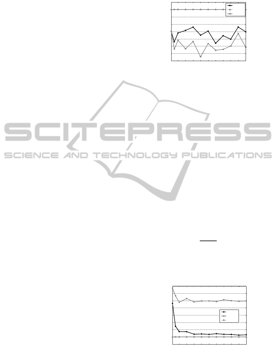
5.1.1 The First Loading Stage (FLS)

This measurement indicates at which stage of the pro-

cess the algorithm began to load items. That is, the

stage in which the DM met its ﬁrst desirable offer.

Figure 1 draws the FLSs with regards to their position

in the selection process. The ﬁgure compares FLS

values obtained by each of the utility functions to the

static case (where FLS is the last stage).

100 200 300 400 500 600 700 800 900 1000

100

110

Problem size

First loading stage (%)

0−1KP

Figure 1: A comparison of FLS values using U

and U

We can see from Table 3 and Figure 1 that FLS

values using the utility functionU

are always greater

than those of U

(except with instance of size 10).

Therefore, wa can say that the utility function U

more convenient for DMs who desire to make deci-

sions in a close time horizon, while U

is more suit-

able for DMs who desire to delay their decisions until

a considerable number of items appears.

5.1.2 The Percentage of Loads Before the Last

Stage (LBLS)

This performance measures assesses the ability of the

algorithm to select desirable items in an online man-

ner. Indeed, when the ﬁnal stage is reached the prob-

lem becomes static (all items are already revealed).

Thanks to the dynamic approach, we can begin to load

items as soon as they appear, and we do not need to

wait until all items are received. LBLS is stated as

follows:

LBLS =

NLIBF

NLI

× 100 (5)

where NLIBF and NLI denote respectively: the

number of loaded items before the ﬁnal stage and the

total number of loaded items. The greater is LBLS,

the more performing the algorithm.

100 200 300 400 500 600 700 800 900 1000

−5

Problem size

LBLS (%)

0−1KP

Figure 2: Comparison of LBLS values using U

and U

Figure 2 reports the LBLS behavior for each of the

used utility functions with regards to the static case.

LBLS values usingU

indicate that the ﬁnal stage still

ICORES2014-InternationalConferenceonOperationsResearchandEnterpriseSystems

218

of a considerable importance regarding the number of

items selected at it: it monopolizesthe biggest propor-

tion of loads. However, the LBLS is higher using U

about 25% of items are loaded before the last stage.

We notice that both curves have similar shapes but the

one of U

is lowest: this is due to the penalty of de-

lay. Indeed,U

penalizes delayed items more severely

than do U

To conclude, we can say that our algorithm has

proved to be efﬁcient in solving the OKP. Compared

with the results provided in the static case, we reached

almost the same overall proﬁts. Besides to respecting

the capacity constraint, we were able to ﬁll at maxi-

mum the knapsack while making decision in oppor-

tune time. As to the utility functions, we noted that

the utility function U

proved to be more convenient

in terms of FLS and LBLS: it gives more interest in

newcomers if compared with U

, which prefers to de-

lay as much as possible and makes decision in latest

stages. However, the utility function does not con-

tribute in the overall reward: we reached all the time

the same values using either functions of utility.

The weak point in our algorithm is its high com-

plexity. As it can be seen in Table 3, the CPU time

is very high and increases exponentially as the size of

the problem increases. We think that this should be

given more attention in future works.

6 CONCLUSIONS

In this paper, we proposed a dynamic approach for

the OKP with delay that incorporates a stopping rule

at each stage of the loading process to enable the DM

to select his best items in an online manner. This ap-

proach was adopted to reduce the OKP to a series

of static knapsack subproblems. Using the optimal

stopping terminology, we stated our decision strategy

based on a dynamic formulation. Experimental re-

sults showed that we were able to reach optimal so-

lution using our online approach. Besides, the use of

two different utility functions allowed us to come up

to the desired solution while involving two different

attitudes to risk.

Future works may include improvements of the

present algorithm in order to reduce the CPU time. A

possible generalization of the present work is to study

the OKP with delay while considering the possibility

of losing a number of items during the selection pro-

cess. The other aspect that we would like to explore

in the future is the OKP with multiple DM.

REFERENCES

Aggarwal, G. and Hartline, J. D. (2006). Knapsack auc-

tions. In SODA ’06: Proceedings of the seventeenth

annual ACM-SIAM symposium on Discrete algorithm,

pages 1083–1092. ACM.

Albers, S. (2003). Online algorithms: a survey. Mathemat-

ical Programming, 97(1-2):3–26.

Babaioff, M., Immorlica, N., Kempe, D., and Kleinberg, R.

(2007). A knapsack secretary problem with applica-

tions. In Approximation, Randomization, and Com-

binatorial Optimization. Algorithms and Techniques,

volume 4627 of Lecture Notes in Computer Science,

pages 16–28.

Gilbert, J. and Mosteller, F. (2006). Recognizing the max-

imum of a sequence. In Selected Papers of Freder-

ick Mosteller, Springer Series in Statistics, pages 355–

398.

Han, X. and Makino, K. (2009). Online knapsack problems

with limited cuts. In Algorithms and Computation,

volume 5878 of Lecture Notes in Computer Science,

pages 341–351. Springer Berlin Heidelberg.

Iwama, K. and Taketomi, S. (2002). Removable online

knapsack problems. In Automata, Languages and

Programming, Lecture Notes in Computer Science,

pages 293–305. Springer Berlin Heidelberg.

Iwama, K. and Zhang, G. (2010). Online knapsack with re-

source augmentation. Inf. Process. Lett., pages 1016–

1020.

Kleywegt, A. J. and Papastavrou, J. D. (1998). The dy-

namic and stochastic knapsack problem. Operations

Research, 46:17–35.

Kramer, A. D. I. (2010). Delaying decisions in order to

learn the distribution of options. PhD thesis.

Lueker, G. S. (1995). Average-case analysis of off-line and

on-line knapsack problems. In SODA ’95: Proceed-

ings of the sixth annual ACM-SIAM symposium on

Discrete algorithms, pages 179–188. Society for In-

dustrial and Applied Mathematics.

Mahdian, M., Nazerzadeh, H., and Saberi, A. (2012). On-

line optimization with uncertain information. ACM

Trans. Algorithms, 8:2:1–2:29.

Marchetti-Spaccamela, A. and Vercellis, C. (1995).

Stochastic on-line knapsack problems. Mathematical

Programming, 68:73–104.

Marini, C., Nicosia, G., Paciﬁci, A., and Pferschy, U.

(2013). Strategies in competing subset selection. An-

nals of Operations Research, 207(1):181–200.

Papastavrou, J. D. and Kleywegt, A. J. (2001). The dynamic

and stochastic knapsack problem with random sized

items. Operations Research, 49:26–41.

Pisinger, D. (1995). An expanding-core algorithm for the

exact 0-1 knapsack problem. European Journal of Op-

erational Research, 87(1):175 – 187.

Zhou, Y., Chakrabarty, D., and Lukose, R. (2008). Budget

constrained bidding in keyword auctions and online

knapsack problems. In Internet and Network Eco-

nomics, volume 5385 of Lecture Notes in Computer

Science, pages 566–576.

OnlineKnapsackProblemwithItemsDelay

219

APPENDIX

Table 3: Comparison of the results provided by the proposed approach in terms of several performance measures.

n NLI AR FLS LBLS (%) CPU

Min 5 5 3507 3507 4 4 0.0 0.0 0.0001

10 Avg 6 6 3848 3825 7 7 23.14 33.57 0.0004

Max 7 7 4202 4202 10 10 33.33 66.66 0.0014

Min 30 30 17884 17884 17 14 3.032 21.87 0.001

50 Avg 32 32 20019 20019 28 23 7.38 28.29 0.017

Max 33 33 23202 23202 43 39 12.5 33.33 0.002

Min 60 60 39332 39332 33 31 1.61 18.03 0.003

100 Avg 62 62 41283 41283 68 58 3.72 23.9 0.011

Max 65 65 42311 42311 97 85 6.15 30 0.015

Min 121 121 78016 78016 93 56 0.81 24.0 0.14

200 Avg 124 124 81557 81557 143 93 3.62 26.43 0.15

Max 127 127 84735 84735 198 172 5.78 29.75 0.17

Min 183 184 118636 118636 122 88 0.0 19.78 0.51

300 Avg 190 190 123109 123110 228 169 1.9 24.11 0.74

Max 197 197 127096 127096 300 215 3.14 25.38 0.80

Min 243 243 154889 154889 133 107 0.4 21.82 1.66

400 Avg 251 251 161030 161031 260 142 2.08 24.71 2.24

Max 257 257 166775 166775 373 184 3.57 29.62 2.65

Min 309 308 191223 191223 223 138 0.63 22.72 2.11

500 Avg 314 314 202696 202696 353 268 1.78 24.84 5.08

Max 320 320 214782 214782 496 389 2.57 26.25 9.41

Min 369 369 235853 235853 210 160 1.89 21.72 4.91

600 Avg 374 374 243081 243081 324 267 2.25 24.38 9.08

Max 383 383 249203 249203 585 501 3.39 27.49 13.01

Min 427 427 271964 271964 236 201 1.15 22.95 12.77

700 Avg 436 436 282368 282368 450 320 1.83 25.65 13.95

Max 445 445 296739 296739 678 480 2.76 27.79 17.60

Min 489 489 314685 314685 267 213 1.43 22.49 13.31

800 Avg 501 501 326031 326031 476 402 1.73 24.97 22.05

Max 516 516 332545 332545 787 737 2.13 25.58 29.50

Min 552 552 358579 358579 312 244 0.9 22.82 34.22

900 Avg 563 563 366009 366009 685 605 1.27 24.59 36.93

Max 576 576 369977 369977 894 871 1.73 25.34 40.79

Min 615 615 400685 400685 340 266 0.48 24.06 47.62

1000 Avg 626 626 410631 410631 696 484 1.5 24.78 54.02

Max 639 639 421587 421587 985 809 2.19 27.69 67.44

ICORES2014-InternationalConferenceonOperationsResearchandEnterpriseSystems

220