
A Case of the Container-Vessel Scheduling Problem
Selim Bora
1
, Endre Boros
2
, Lei Lei
3
, W. Art Chaovalitwongse
4
, Gino J. Lim
5
and Hamid R. Parsaei
1
1
Mechanical Engineering, Texas A&M University at Qatar, Doha, Qatar
2
RUTCOR, Rutgers University, New Jersey, U.S.A.
3
SCMMS, Rutgers University, New Jersey, U.S.A.
4
Industrial&Systems Engineering, University of Washington, Washington, U.S.A.
5
Industrial Engineering, University of Houston, Texas, U.S.A.
Keywords:
Vessel Scheduling, Bender’s Decomposition, Dynamic Programming.
Abstract:
We study a difficult real life scheduling problem encountered in oil and petrochemical industry, involving in-
ventory and distribution operations, which requires integrated scheduling. The problem itself is NP-complete,
however we show some special cases, and propose polynomial time solution methods. These could be used
as a starting point for a heuristic making use of these simplified cases. This study proposes two alternative
approaches for the main problem, one of them making use of one of the special cases using minimum cost
flow formulation, and the other one using Benders Decomposition once the problem is reformulated to make it
easier to handle. Both results show promising results and computation time. Benders Decomposition approach
allows exact solutions to be found in a much faster fashion.
1 INTRODUCTION
This study is focused on the demand-supply coordina-
tion problem encountered in petrochemical industry
such as oil and gasoline. The cost to produce and de-
liver gasoline products to the market consists of three
major components: the transportation cost of crude
oil to refiners, the operation cost of refinery process-
ing, and the cost of marketing and distribution. An
oil company typically operates many tens of refiner-
ies, with several million barrels of crude oil per day
and several billion dollars on crude transportation per
year. As the retail gasoline prices continue to rapidly
elevate around the world, effectively coordinating the
demand and supply of gasoline products has there-
fore become even more crucial to oil companies. Par-
ticularly in this study, the company uses its own and
chartered vessels to distribute the gasoline products to
discharging/demand locations. Each discharging lo-
cation carries its own inventories and serves as a de-
pot of distribution for the local market. Since vessels
are expensive in both variable and fixed costs, any in-
efficiency in the supply process could result in a sub-
stantial operating cost. The distribution scheduling
problem encountered in this process is very compli-
cated due to the involvement of heterogeneous vessels
(e.g., in terms of their loading capacities, discharging
and berthing times, and operating costs) and the fact
that each vessel has multi-level of loading capacities
such that a load beyond the normal/base capacity will
result in an extra overload cost. Practical issues faced
include which vessel should deliver to which depot
in which time period, whether a particular vessel trip
should carry an extra load and by how much, and what
should be the ending inventory at a depot in a par-
ticular period, etc. Due to high distribution cost of
gasoline products, an effectively distribution schedule
could help the company to further improve the profit
of its supply chain and to strengthen its competitive
advantage in the market place.
Our goal is to minimize the operating costs related
to shipping and handling of goods. The fleet size is
not fixed, nor an initial amount is set, so one of the
tasks we have at hand is to determine the number of
vessels that will be used within the planning horizon.
Shipping costs can be divided into two categories:1)
The fixed cost related to either purchase or lease of a
vessel, 2) the overloading cost which is incurred if the
vessels carry above a certain capacity. There are two
more costs that we need to watch out for. Each ship-
ment made to a port may incur a holding or penalty
cost based on the demand. If the demand is not met
63
Bora S., Boros E., Lei L., Art Chaovalitwongse W., J. Lim G. and R. Parsaei H..
A Case of the Container-Vessel Scheduling Problem.
DOI: 10.5220/0004831400630071
In Proceedings of the 3rd International Conference on Operations Research and Enterprise Systems (ICORES-2014), pages 63-71
ISBN: 978-989-758-017-8
Copyright
c
2014 SCITEPRESS (Science and Technology Publications, Lda.)

on time, it cannot be satisfied at a later time period,
and therefore we need to pay penalty for each unit.
Also, if the port is forced to hold some inventory, then
a holding cost is charged. In addition to all these cost
factors, we also need to consider the fact that each
vessel is available for a certain amount of time within
a period, and therefore even if a vessel has enough
capacity, it may not have enough time to visit all the
ports we desire.
Optimally solving distribution operations schedul-
ing problem is not an easy task. Previous work related
to industrial shipping varies a lot. Here, we focus
on the existing results that are closely related to our
work. A large summary of works related to various
types of vessel scheduling and routing problem can be
found in the literature survey by (Christiansen et al.,
2004). Two more recent surveys can be found more
specifically in the area of combined inventory man-
agement and routing ((Andersson et al., 2010)) and
on fleet composition and routing ((Hoff et al., 2010)).
The most recent literature survey is by (Christiansen
et al., 2012), which takes a look at the publications in
the last decade, and list possible research areas that
could be pursued in this area.
(Xinlian et al., 2000) presents an algorithm which
combines the linear programming technique with that
of dynamic programming to improve the solution to
linear model for fleet planning. Even though their ap-
proach is similar, the problem they are dealing with
requires demand satisfaction and initial fleet is al-
ready given, and the decision is to whether add new
vessels to the existing fleet or not.
(Cho and Perakis, 2001) presented a better formu-
lation to the original fleet deployment problem pro-
posed by (Ronen, 1986). In this formulation, just like
we do, there is a single loading port, finite number of
customer ports, and a finite planning horizon. How-
ever, they require the demand to be met, and the fleet
size is constant. The costs incurred are due to routes
chosen, shipping cargoes, and unloading time. They
show that this formulation is better for computational
efficiency.
(Cho and Perakis, 1996) present a study regarding
fleet size and design of optimal liner routes for a con-
tainer shipping company. The problem is solved by
generating a number of candidate routes for the dif-
ferent ships first, and then, the problem is formulated
and solved as a linear programming model, where the
columns represent the candidate routes. They extend
this model to a mixed integer programming model
that also considers investment alternatives to expand-
ing fleet capacity. (Bendall and Stent, 2001) also
present a model for determining the optimal number
of ships and fleet deployment plan.
On the other hand, (Nicholson and Pullen, 1971)
were the first ones to propose dynamic programming
application to ship fleet management. The problem
they dealt with was to determine the sequence in
which the currently owned ships should be sold and
the extent to which charter ships should be taken on.
They tackle the problem in two stages. The first stage
determines a good priority ordering for selling the
ships regardless of the rate at which charter ships are
taken on. The second stage uses dynamic program-
ming to determine an optimal level of chartering given
the priority replacement order. This first stage pri-
ority ordering essentially reduces the dynamic pro-
gramming calculation from a problem with as many
as states as number of ships in fleet to a 1 state vari-
able problem which is computationally manageable
by dynamic programming methods. Several authors
use benchmark instances to compare the results of
different strategies and heuristics. (Gheysens et al.,
1984) define 20 test instances with 12100 nodes for
the standard fleet size and mix vehicle routing prob-
lem. (Wu et al., 2005) deals with trucks that vary in
capacity and age are utilized over space and time to
meet customer demand. Operational decisions (in-
cluding demand allocation and empty truck reposi-
tioning) and tactical decisions (including asset pro-
curements and sales) are explicitly examined in a lin-
ear programming model to determine the optimal fleet
size and mix. The method uses a time-space network,
common to fleet-management problems, but also in-
cludes capital cost decisions, wherein assets of dif-
ferent ages carry different costs, as is common to re-
placement analysis problems. A two-phase solution
approach is developed to solve large-scale instances
of the problem. Phase I allocates customer demand
among assets through Benders decomposition with a
demand-shifting algorithm assuring feasibility in each
subproblem. Phase II uses the initial bounds and dual
variables from Phase I and further improves the so-
lution convergence through the use of Lagrangian re-
laxation.
A network optimization approach has been
proposed by (Bookbinder and Reece, 1988), where
they formulate a multi-commodity capacitated
distribution-planning problem as a non-linear mixed
integer programming model, and solve it as a gener-
alized assignment problem within an algorithm for
the overall distribution/routing problem based on a
Bender’s type decomposition.
(Lei et al., 2009) proposes an approach to a bi-
directional flow problem where each iteration starts
with a given planning horizon, which is then parti-
tioned into three planning intervals, where each inter-
val consists of consecutive time periods in the given
ICORES2014-InternationalConferenceonOperationsResearchandEnterpriseSystems
64

planning horizon. Afterwards, some constraint relax-
ations are applied to the problem in which all the for-
ward demand and all the backward demand of the
time periods in the third planning interval are con-
solidated into a single forward demand and a single
backward demand, which is an idea we use in one of
our approaches.
(Choi et al., 2012) focuses on minimizing total tar-
diness, rather than the operating costs, and the routes
for vessels are observed under three different cases,
one of them being arbitrary, just like in our problem.
Later on, they talk about the other problems in the lit-
erature and how their approach is related to them.
2 PROBLEM DEFINITION
This paper, brings together some of the ideas that
were proposed in the literature before. We are given
a fleet |V | of container vessels, v ∈ V that distributes
the goods from a main distribution center to a
number of customer ports over a |T |-period planning
horizon. Each vessel has two loading capacities:
the regular loading capacity u
0
v
, and the maximum
loading capacity u
max
v
so that carrying a load beyond
u
0
v
will impose an over loading charge g
0
v
/unit and
carrying a load beyond u
max
v
violates the feasibility.
In addition to this limitation, for every vessel there
is total available time τ
v
which is used up by the
berthing time b
v,p
at ports which vary depending
on vessel type. There are |p| customer ports on the
network, each port p ∈ P has a demand, d
p,t
≥ 0
in period t ∈ T. For every port, unsatisfied demand
are penalized at p
p,t
/unit based on the unsatisfied
demand and no backlogging is allowed. On the
other hand, end of period inventory incurs a holding
cost of h
n
/unit. Let c
f
v
denote the fixed cost if the
vessel is being dispatched in a period. The problem
is finding a feasible vessel dispatching schedule to
minimize the total shortage and overage penalty plus
the vessel overloading and fixed cost.The minimum
cost flow network formulation proposed guarantees
optimality when the number of vessels dispatched in
every period is known. To define our problem more
formally, we define the following set of variables:
S
p,t
∈ Z
+
: amount of shortage at port p in period t
Q
v,p,t
∈ Z
+
: amount of supply delivered to port p in
period t via vessel v’s regular capacity
O
v,p,t
∈ Z
+
: amount of supply delivered to port p in
period t via vessel v’s overloading capacity
I
p,t
∈ Z
+
: ending inventory at port p in period t
Y
v,p,t
∈ {0,1}: Y
v,n,t
= 1 if vessel v delivers to port p
in period t
Z
v,t
∈ {0,1}: Z
v,t
= 1 if vessel v is dispatched in
period t
Based on this, the constraints to the problem will
include the following:
A vessel must not be carrying anything if it’s not
dispatched, nor visiting ports:
Q
v,p,t
+ O
v,p,t
≤ u
max
v
Y
v,p,t
∀ v ∈ V, p ∈ P, t ∈ T
(1a)
Y
v,p,t
≤ Z
v,t
∀ v ∈ V, p ∈ P, t ∈ T
(1b)
Vessels dispatched must not be used over their
time and regular/maximum capacity:
∑
p∈P
b
v,p
Y
v,p,t
≤ τ
v
∀ v ∈ V, t ∈ T (2a)
∑
p∈P
Q
v,p,t
≤ u
0
v
∀ v ∈ V, t ∈ T (2b)
∑
p∈P
(Q
v,p,t
+ O
v,p,t
) ≤ u
max
v
∀ v ∈ V, t ∈ T (2c)
The last group of constraints is to help to formu-
late our objective, which is a compositions of all ex-
penses (penalties, etc.).
Vessel dispatching costs:
c
D
=
∑
v∈V
∑
t∈T
c
f
v
Z
v,t
(3a)
Early arrival penalties:
c
H
=
∑
p∈P
∑
t∈T
h
p
I
p,t
(3b)
Unsatisfied demands’ penalties:
c
U
=
∑
p∈P
∑
t∈T
p
p,t
S
p,t
(3c)
Overloading penalties:
c
O
=
∑
v∈V
∑
p∈P
∑
t∈T
g
0
v
O
v,p,t
(3d)
Then our problem is to minimize c
D
+ c
H
+ c
U
+
c
O
, subject to the constraints (1)-(3) and the sign and
type restrictions in the definitions of the decision vari-
ables.
If the dispatching information is already available,
i.e. |V
1
| vessels for t=1, |V
2
| for t=2, . . . , |V
T
| for t=T,
then there becomes no need for the binary variables.
In addition, define new variables, x
v,k,n,t
and r
v,k,n,t
,
which are the normal and over flows shipped by ves-
sel v dispatched in period k for port n to satisfy the
ACaseoftheContainer-VesselSchedulingProblem
65
demand on period t. Based on this definition, the fol-
lowing can be established:
Q
v,p,t
=
T
∑
k=t
x
v,t,p,k
∀ v ∈ V, p ∈ P, t ∈ T (4a)
O
v,p,t
=
T
∑
k=t
r
v,t,p,k
∀ v ∈ V, p ∈ P, t ∈ T (4b)
S
p,t
= d
p,t
−
∑
k∈T
∑
v∈V
k
(x
v,k,p,t
+ r
v,k,p,t
)
∀ p ∈ P, t ∈ T (4c)
I
p,t
=
∑
k∈T
T
∑
w=t+1
∑
v∈V
k
(x
v,k,p,w
+ r
v,k,p,w
)
∀ p ∈ P, t ∈ T (4d)
Based on the above assumptions and definitions, we
get the following model. Objective function is the
same except that the last part is now a constant based
on vessel dispatching information, i.e. Z
v,t
values are
known. Constraints (5b) and (5c) assure that normal
and over capacity are not exceeded, where as con-
straint (5d) prevents shipments for a specific demand
to be more than the demand itself, therefore making
the first part of the objective function always nonneg-
ative.
min
∑
p∈P
∑
t∈T
p
p,t
(d
p,t
−
T
∑
k=1
∑
v∈V
k
(x
v,k,p,t
+ r
v,k,p,t
))
+
∑
v∈V
∑
p∈P
∑
t∈T
g
0
v
T
∑
k=t
r
v,t,p,k
+
∑
v∈V
∑
t∈T
c
f
v
Z
v,t
+
∑
p∈P
∑
t∈T
h
p
t
∑
k=1
T
∑
w=t+1
∑
v∈V
k
(x
v,k,p,w
+ r
v,k,p,w
)
(5a)
s.t.
∑
p∈P
b
v,p
Y
v,p,t
≤ τ
v
∀ v ∈ V, t ∈ T (5b)
T
∑
k=t
∑
n∈N
(x
v,t,n,k
+ r
v,t,n,k
) ≤ u
max
v
∀ v ∈ V, t ∈ T
(5c)
T
∑
k=t
x
v,t,n,k
+ r
v,t,n,k
≤ u
max
v
Y
v,n,t
∀ v ∈ V, p ∈ P, t ∈ T (5d)
∑
n∈N
T
∑
k=t
x
v,t,n,k
≤ u
0
v
∀ v ∈ V, t ∈ T (5e)
t
∑
k=1
∑
v∈V
k
(x
v,k,n,t
+ r
v,k,n,t
) ∀ p ∈ P, t ∈ T (5f)
Y
v,n,t
≤ Z
v,t
∀ v ∈ V, p ∈ P, t ∈ T (5g)
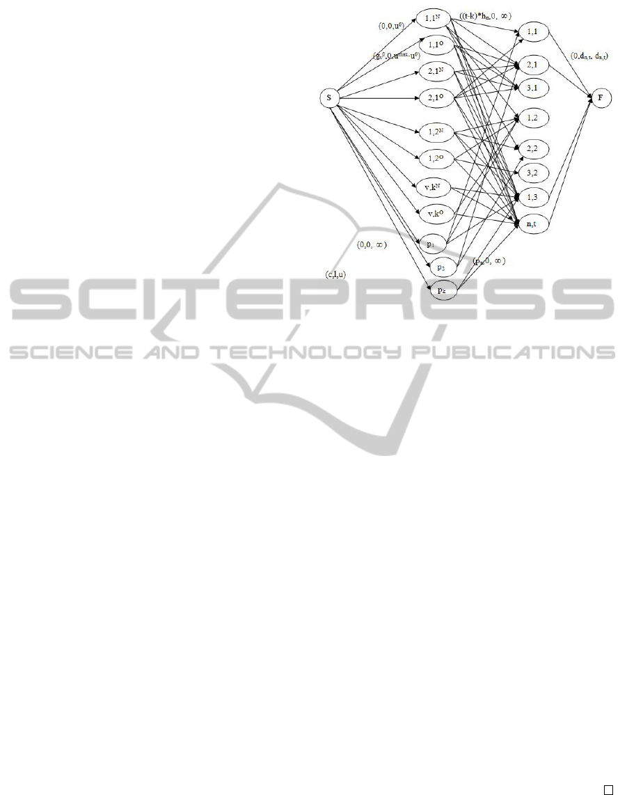
Figure 1: An example of the network for |V
1
| = 2, |V
2
| = 1,
|V
3
| = 2, |N| = 3, and |T | = 3.
Lemma 2.1. The above problem can be reformulated
without the berthing time constraint and solved as a
minimum cost flow problem by assuming the knowl-
edge of the number of vessels dispatched in each time
period.
Proof. First, we construct a dummy source node S,
and a dummy sink node F. Associate to each vessel
v ∈ V
k
, 2 nodes (v,k)
P
and (v,k)
O
, one for normal and
other for over capacity. These nodes are connected to
the source node with 0 and g
0
v
costs, a lower bound of
0 and an upper bound u
0
v
and u
max
v
− u
0
v
respectively.
Add another set of |P| nodes (p
p
) for case of short-
age at each port with 0 costs, 0 lower bounds and no
upper bounds. Next, take care of the ports by adding
|P| ∗ |T | nodes denoted (p,t) for each port n at every
period t. The arcs between nodes corresponding to
vessels and ports incur a holding cost of h
p
(t −k), has
a lower bound of 0 and no upper bound. Also, there
will be arcs between shortage nodes, (p
p
), and ports,
(p,t), where the shortage costs p
p,t
will be charged.
Finally, add arcs between ports and the sink, with a
lower and upper bound of d
p,t
and no cost.This net-
work will have 2|V ||T |+|P|+|P||T | many nodes, and
|V ||P||T
2
| + |P
2
| many arcs, making minimum cost
flow approach practical for problems of reasonable
size. An example network is shown in Figure 1.
Lemma 2.2. The objective function values and con-
straints for both problems above are the same, assum-
ing we guessed the right number of vessels.
ICORES2014-InternationalConferenceonOperationsResearchandEnterpriseSystems
66

Proof. First of all, the fixed cost due to vessels for
both problems will be the same. Next, assume x
∗
v,k,n,t
and r
∗
v,k,n,t
are the optimal flow vectors correspond-
ing to the minimum cost flow problem. Then, us-
ing the equalities corresponding the variables of two
problems, the objective function value of the original
problem becomes:
∑
p∈P
∑
t∈T
p
p,t
(d
p,t
−
∑
k∈T
∑
v∈V
k
(x
v,k,p,t
+ r
v,k,p,t
))+
∑
v∈V
∑
p∈P
∑
t∈T
g
0
v
∑
T
k=t
r
v,t,p,k
+
∑
v∈V
∑
t∈T
c
f
v
Z
v,t
+
∑
p∈P
∑
t∈T
h
p
∑
k∈T
∑
T
w=t+1
∑
v∈V
k
(x
v,k,p,w
+ r
v,k,p,w
)
=
∑
p∈P
∑
t∈T
p
p,t
S
∗
p,t
+
∑
v∈V
∑
p∈P
∑
t∈T
g
0
v
O
∗
v,k,p,t
+
∑
v∈V
∑
t∈T
c
f
v
Z
∗
v,t
+
∑
p∈P
∑
t∈T
h
p
I
∗
p,t
(6)
The first 2 lines of this equality (6) and the objective
function of the minimum cost flow are exactly the
same, which only leaves us with the inventory part.
The w index is for shipments that are on a future date
than current period t, and the k index is taking into
account all shipments that have been made up to pe-
riod t. Therefore, a shipment made on period k for
period t will appear in the summation (t − k) many
times, allowing us to replace index w with t, remove
the summation regarding w, and charge the holding
cost as many times as necessary. This shows that both
objective function values are the same.
As far as the constraints are concerned, first re-
alize that in the original problem, (2a) is no longer
required while berthing times are large enough. Sim-
ilarly, (1a) and (1b) were associated with the fact that
dispatching information was not available, so now,
they could be dropped as well. (2b) in the original
problem is the same constraint as (5d) in the reduced
problem, and they are both concerned with normal ca-
pacity of a vessel. (5c) and (5d) of the reduced prob-
lem, added together, imply the same restriction on
maximum vessel capacity as (2c) of the original prob-
lem. On the other hand, the flow balance constraint in
the original problem is taken care of by two means:
1) the new index k for the variables, tells us when
shipment was made, so we now whether a shipment
is held at inventory or used immediately, 2) in the re-
duced problem, shipment for a specific demand will
not be more than the demand itself, therefore short-
age never becomes negative according to the relation
between S
n,t
and x
v,k,n,t
, r
v,k,n,t
.
3 SPECIAL CASES
Figure 2 is a list of special cases deduced from the
general problem, for which we propose efficient so-
lution approaches. Case 7 makes use of the method
proposed by (Detti, 2009), used for solving knapsack
problems with divisible item sizes.
Based on our minimum cost network flow ap-
proach, we propose the following two heuristics for
no berthing time case:
3.1 Backward Heuristic
1. Divide the planning horizon into two groups, pri-
mary and secondary, for each port, the new de-
mand is equal to sum of the individual demands
in each group, holding cost is the minimum and
penalty cost is the maximum of individual penal-
ties.
2. Start with |P| ∗ |T | vessels in that group in total,
solve the minimum cost flow problem iterating
through all vessel dispatching combinations avail-
able for a group.
3. Once the optimal number of vessels required for
each group are determined, repeat the procedure
of dividing into groups and solving as a minimum
cost flow problem for the individual groups. De-
mand belonging to ports in the other individual
group is also added to the demand of the ports in
the secondary period of the group under consider-
ation.
4. Once the primary group has only 1 period remain-
ing, optimal number of vessels have been deter-
mined for that group, start over.
3.2 Greedy Heuristic
1. Start with no vessels assigned to each period.
2. Add a vessel to any period and solve the prob-
lem. Remove the vessel, and add to another pe-
riod, and solve again. Once the best vessel addi-
tion has been determined, move on to next vessel
addition.
3. Keep determining the best vessel to add until ob-
jective function no longer improves.
Going back to the original problem with berthing con-
straints, we propose modified greedy heuristics and
a decomposition based exact method. We first intro-
duce the algorithms and then compare them with state
of the are integer programming solver, XpressMP.
3.3 Improved Greedy Heuristic
1. Start with no vessels assigned to each period.
ACaseoftheContainer-VesselSchedulingProblem
67
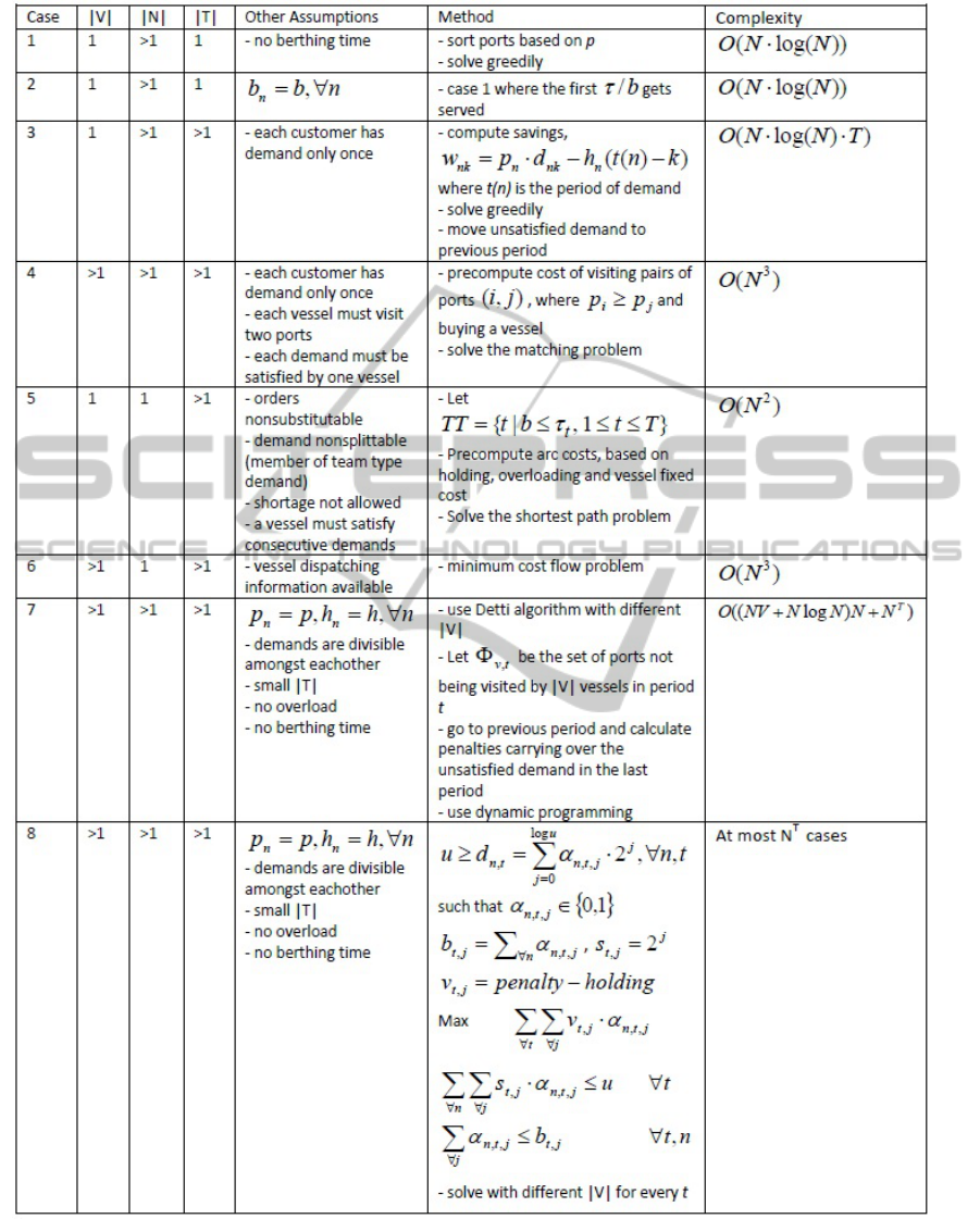
Figure 2: Special cases deduced from the general problem under different assumptions.
2. For each vessel type, compute maximal subsets of
ports such that no further port can be added to a
set due to berthing time constraint.
3. For each vessel type, in every period, sort the
subset of ports in decreasing order based on
∑
n∈Maximal
v
d
n,t
p
n,t
ICORES2014-InternationalConferenceonOperationsResearchandEnterpriseSystems
68
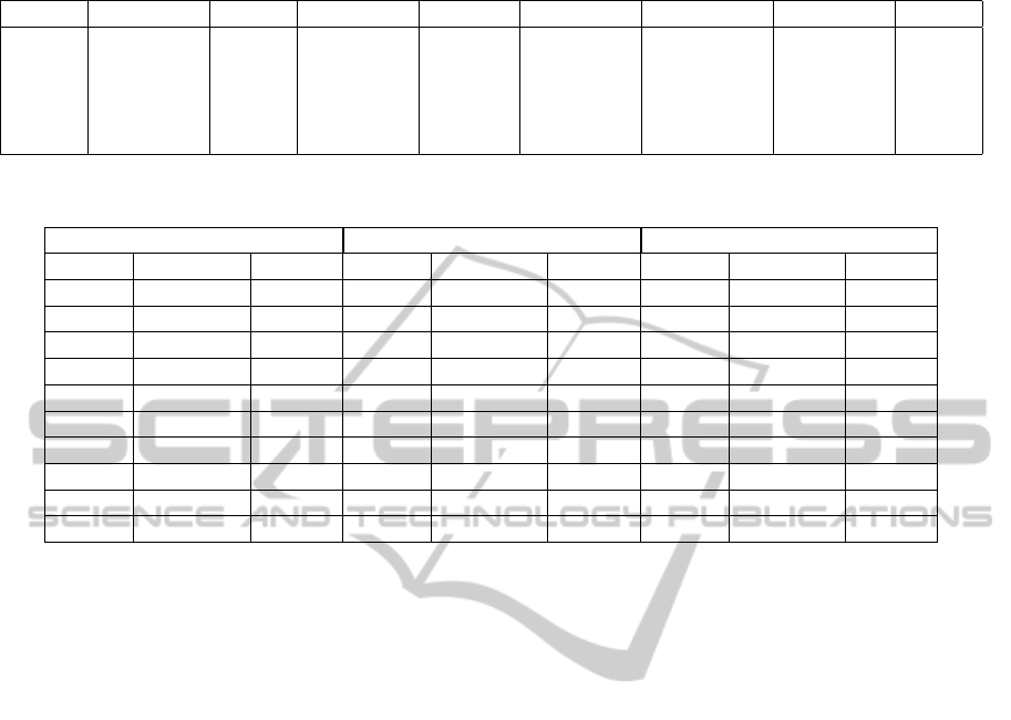
Table 1: |N|=3, |T |=4, vessel type same, number of vessels in each period shown, as well as the optimal objective function
value for each case, indicating that even a much simpler version of the original problem is not submodular.
Case 1 Obj. Func. Case 2 Obj. Func. Case Int Obj. Func. Case Union Obj. Func. Comp.
(3,2,2) 170 (2,1,3) 390 (2,1,2) 540 (3,2,3) 50 Lower
(1,2,1) 840 (2,1,3) 390 (1,1,1) 1140 (2,2,3) 90 Equal
(2,2,1) 580 (2,1,3) 390 (2,1,1) 880 (2,2,3) 90 Equal
(1,2,3) 350 (2,1,3) 390 (1,1,3) 650 (2,2,3) 90 Equal
(1,3,2) 390 (2,1,3) 390 (1,1,2) 800 (2,3,3) 50 Lower
Table 2: |N|=10, |T |=10, 3 different vessel types, number of vessels each method solves for vary for XpressMP, Backward
and Greedy as 10, 100, 1 in respect. Runs are terminated after 2 hours or when 0.1% gap from the best bound is reached.
Time (sec) Objective Function Gap (%)
Xpress Backward Greedy Xpress Backward Greedy Xpress Backward Greedy
7200 412.50 435.8 7503 7799 7733 1.7384 5.47 4.66
7200 420.40 435.20 8141 8314 8298 2.1557 4.20 4.01
7200 393.30 420.60 8270 8483 8450 0.9988 3.48 3.11
7200 332.30 390.70 7759 7806 7800 0.3519 0.95 0.88
7200 289.90 316.80 7316 7395 7375 0.1414 1.20 0.94
7200 310.30 336.60 8412 8494 8487 3.2309 4.16 4.09
7200 345.2 347.6 8270 8356 8338 3.8278 4.82 4.62
7200 429.50 443.30 7918 8159 8112 1.1641 4.08 3.53
7200 421.8 425.8 7475 7825 7768 1.4574 5.87 5.17
7200 306.70 321.10 7448 7661 7600 2.4489 5.16 4.40
4. Next, add any vessel to any period allowing it to
only serve the top ranked subset of ports and solve
the problem. Try different vessel types, for differ-
ent periods in the same manner. Determine the
best vessel to add to which period.
5. Once a vessel assignment has been determined,
update remaining demand and sort subsets of
ports accordingly.
6. Keep determining the best vessel to add until ob-
jective function no longer improves.
3.4 Bender’s Type Decomposition
Approach
1. Choose a feasible assignment of ports to a vessel
to start with.
2. Solve the master problem to obtain a new objec-
tive function value and new port assignments to
other vessels.
3. Keeping port assignments fixed, solve the dual
problem.
4. STOP, if master and dual objective values are
close enough, otherwise go back to the master
problem.
4 COMPUTATIONAL RESULTS
With the minimum cost flow network formulation
proposed, one question that arose was whether it
was worth investing more resources into finding a
dispatching information, and maybe go from there.
However, as can be seen at 1, the minimum cost
flow problem is not submodular. Case 1 and Case 2
are random dispatches, where as Case Int refers to
the scenario where minimum of number of vessels
dispatched in each latter case is used, and Case
Union refers to of Case 1 and Case 2 are random
dispatches, where as Case Int refers to the scenario,
where minimum of number of vessels dispatched in
each latter case is used, and Case Union refers to
the scenario, where maximum of number of vessels
dispatched in each latter case is used.
Backward and Greedy Heuristic both performed
well, however, as can be seen in Table 2, Backward
Heuristic always takes shorter, where as Greedy
Heuristic performs better by a slight margin.
However, it must be kept in mind that Table 2
reflects results for the version of the problem with no
berthing time constraint. Improved Greedy Heuristic
designed to deal with this issue performs a bit slower
than the previously mentioned heuristics, but gives
good bounds for the solution of the original problem
as can be seen in Table 3.
ACaseoftheContainer-VesselSchedulingProblem
69
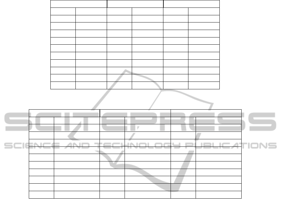
Table 3: |N|=10, |T |=10, 3 different vessel types, number of vessels each method solves for vary for XpressMP and Improved
Greedy as 10 and 1 in respect. All runs are terminated after 2 hours or when 0.1% gap from the best bound is reached.
Time (sec) Objective Function Gap (%)
Xpress I. Greedy Xpress I. Greedy Xpress I. Greedy
7200 593.9 7503 7533 1.74 2.13
7200 582.2 8141 8226 2.16 3.17
7200 635.3 8270 8381 1.00 2.31
7200 678.2 7759 7921 0.35 2.39
7200 668.6 7316 7436 0.14 1.75
7200 594.4 8412 8548 3.23 4.77
7200 649.3 8270 8353 3.83 4.78
7200 667.3 7918 8092 1.16 3.29
7200 641.1 7475 7513 1.46 1.96
7200 662.1 7448 7565 2.45 3.96
Table 4: |N|=10, |T |=10, 3 different vessel types, number of vessels each method solves for vary for XpressMP and Improved
Greedy as 10 and 1 in respect. All runs are terminated after 2 hours or when 0.1% percent gap from the best bound is reached.
Time (sec) Objective Function Gap (%)
Xpress Decomposition Xpress Decomposition Xpress Decomposition
7200 767.1 7503 7380 1.74 0.10
7200 757.5 8141 7973 2.16 0.10
7200 905.8 8270 8196 1.00 0.10
7200 1291.4 7759 7739 0.35 0.10
7200 1420.4 7316 7313 0.14 0.10
7200 959 8412 8148 3.23 0.10
7200 1183.5 8270 7961 3.83 0.10
7200 907.4 7918 7834 1.16 0.10
7200 1032.8 7475 7373 1.46 0.10
7200 1349.4 7448 7273 2.45 0.10
The formulation proposed for Bender’s type ap-
proach is computationally efficient, as can be on Ta-
bles 4 and 5. The running time is a bit longer, but
we’re able to get exact solutions.
5 CONCLUSIONS
In this study, we studied a difficult real life sup-
ply chain scheduling problem encountered in oil and
petrochemical industry, which involves production,
inventory, and distribution operations, and requires
an integrated scheduling to minimize the total oper-
ation cost. We showed the hardness of this prob-
lem, and showed that some of its special cases are
polynomial time solvable. A minimum cost flow
based heuristic, motivated by the observations from
one of the special cases, was proposed and demon-
strated to have a promising performance under the
set of test cases considered in this study. Also, a
new formulation of the model was developed, which
made Bender’s type decomposition method computa-
tionally efficient. Therefore, we’re now able to get
really good(exact) results for big problems at a much
faster fashion then solver XpressMP.
There are several interesting extensions of the
work presented here. These include integrating the
inland production with single or multiple refineries at
different locations on the network, and multiple prod-
ucts needed by the same customer port. This inte-
gration would cause the supply chain to become big-
ger, and therefore more complex, however closer to
reality, as inland production and demand satisfaction
are activities that need synchronization. Furthermore,
the involvement of multiple refineries and multiple
products introduces the new optimization issues due
to assigning refineries to customer ports and allocat-
ing vessel capacity for different products. This will
make the modeling and the design of search proce-
dures more interesting and challenging.
Also, for the simplicity of modeling, in this study,
we assumed a linear penalty function for vessel over-
loading. However, this penalty cost is in reality very
complex and is affected by many factors such as the
level of overloading and navigation conditions. A
nonlinear cost function would be more meaningful in
this case.
ICORES2014-InternationalConferenceonOperationsResearchandEnterpriseSystems
70
Table 5: |N|=15, |T |=10, 3 different vessel types, number of vessels each method solves for vary for XpressMP and Improved
Greedy as 10 and 1 in respect. All runs are terminated after 2 hours or when 0.1% percent gap from the best bound is reached.
Time (sec) Objective Function Gap (%)
Xpress Decomposition Xpress Decomposition Xpress Decomposition
7200 805 7764 7619 1.98 0.10
7200 777.9 8652 8448 2.46 0.10
7200 990.5 8326 8245 1.07 0.10
7200 1401.1 8001 7978 0.39 0.10
7200 1544.6 7464 7461 0.15 0.10
7200 1015.4 8789 8496 3.43 0.10
7200 1216.9 9423 9026 4.30 0.10
7200 984.8 8128 8035 1.24 0.10
7200 1114.2 7849 7727 1.66 0.10
7200 1413.5 7652 7455 2.67 0.10
ACKNOWLEDGEMENTS
This report was made possible by a National Priori-
ties Research Program grant from the Qatar National
Research Fund (a member of The Qatar Foundation).
The statements made herein are solely the responsi-
bility of the authors.
REFERENCES
Andersson, H., Hoff, A., Christiansen, M., Hasle, G.,
and Løkketangen, A. (2010). Industrial aspects and
literature survey: Combined inventory management
and routing. Computers & Operations Research,
37(9):1515–1536.
Bendall, H. and Stent, A. (2001). A scheduling model for
a high speed containership service: A hub and spoke
short-sea application. International Journal of Mar-
itime Economics, 3(3):262–277.
Bookbinder, J. and Reece, K. (1988). Vehicle routing con-
siderations in distribution system design. European
Journal of Operational Research, 37(2):204–213.
Cho, S. and Perakis, A. (1996). Optimal liner fleet route-
ing strategies. Maritime Policy and Management,
23(3):249–259.
Cho, S. and Perakis, A. (2001). An improved formulation
for bulk cargo ship scheduling with a single loading
port. Maritime Policy & Management, 28(4):339–345.
Choi, B., Lee, K., Leung, J., Pinedo, M., and Briskorn, D.
(2012). Container scheduling: Complexity and al-
gorithms. Production and Operations Management,
21(1):115–128.
Christiansen, M., Fagerholt, K., Nygreen, B., and Ronen, D.
(2012). Ship routing and scheduling in the new mil-
lennium. European Journal of Operational Research.
Christiansen, M., Fagerholt, K., and Ronen, D. (2004).
Ship routing and scheduling: Status and perspectives.
Transportation Science, 38(1):1–18.
Detti, P. (2009). A polynomial algorithm for the multiple
knapsack problem with divisible item sizes. Informa-
tion Processing Letters, 109(11):582–584.
Gheysens, F., Golden, B., and Assad, A. (1984). A compar-
ison of techniques for solving the fleet size and mix
vehicle routing problem. OR Spectrum, 6(4):207–216.
Hoff, A., Andersson, H., Christiansen, M., Hasle, G., and
Løkketangen, A. (2010). Industrial aspects and litera-
ture survey: Fleet composition and routing. Comput-
ers & Operations Research, 37(12):2041–2061.
Lei, L., Zhong, H., and Chaovalitwongse, W. (2009). On the
integrated production and distribution problem with
bidirectional flows. INFORMS Journal on Comput-
ing, 21(4):585–598.
Nicholson, T. and Pullen, R. (1971). Dynamic program-
ming applied to ship fleet management. Operational
Research Quarterly, pages 211–220.
Ronen, D. (1986). Short-term scheduling of vessels for
shipping bulk or semi-bulk commodities originating
in a single area. Operations Research, 34(1):164–173.
Wu, P., Hartman, J., and Wilson, G. (2005). An integrated
model and solution approach for fleet sizing with het-
erogeneous assets. Transportation Science, 39(1):87–
103.
Xinlian, X., Tengfei, W., and Daisong, C. (2000). A dy-
namic model and algorithm for fleet planning. Mar-
itime Policy & Management, 27(1):53–63.
ACaseoftheContainer-VesselSchedulingProblem
71
