A First Algorithm to Calculate Force Histograms in the Case of
3D Vector Objects
Jameson Reed, Mohammad Naeem and Pascal Matsakis
School of Computer Science, University of Guelph, Kemptville, ON K0G 1J0, Canada
Keywords: Relative Positions, Spatial Relationships, Polygon Meshes.
Abstract: In daily conversation, people use spatial prepositions to denote spatial relationships and describe relative
positions. Various quantitative relative position descriptors can be found in the literature. However, they all
have been designed with 2D objects in mind, most of them cannot be extended to handle 3D objects in vec-
tor form, and there is currently no implementation able to process such objects. In this paper, we build on a
descriptor called the histogram of forces, and we present the first algorithm for quantitative relative position
descriptor calculation in the case of 3D vector objects. Experiments validate the approach.
1 INTRODUCTION
In daily conversation, people use spatial prepositions
to denote spatial relationships and describe relative
positions (e.g., the apple in the bowl, the bowl near
the vase, the vase in front of the window). Most
research on relative position descriptors and models
of spatial relationships has focused so far on quali-
tative approaches and 2D objects (or 2D perspec-
tives of 3D objects), often with the assumption that
the objects were far enough from each other and
could be approximated by their centres or minimum
bounding rectangles. Unacceptable processing times,
human cognitive limitations, a strong inhibitor factor
(our long history with 2D research), the ubiquity of
2D data and the increased complexity of 3D model-
ling have channelled the researchers’ attention away
from quantitative approaches, 3D objects and intri-
cate configurations. In the past few years, however,
computer processing speed as well as storage and
memory capacity have kept improving at exponen-
tial rates, technical limitations to the handling of 3D
spatial data have been decreasing, and there has been
a surge of wide-ranging interest in 3D contents.
In this paper, we present what we believe is the
first algorithm for quantitative relative position de-
scriptor calculation in the case of 3D objects in vec-
tor form. Various descriptors can be found in the
literature (Miyajima and Ralescu, 1994); (Wang and
Makedon, 2003); (Kwasnicka and Paradowski, 2005);
(Zhang et al., 2010). As far as we know, however,
they all have been designed with 2D objects in mind
(mainly objects in raster form), most of them cannot
be extended to handle 3D vector objects, and there is
currently no implementation able to process such
objects. After a thorough comparative analysis, we
have chosen to build on a descriptor called the histo-
gram of forces (Matsakis et al., 2011). Its math-
ematical definition holds in any Euclidean space,
and theory endows it with remarkable properties. It
is able to handle a variety of objects (e.g., connected
or disconnected, with or without holes, disjoint or
intersecting). Its behaviour towards affine transfor-
mations is known. It can easily be normalized to
achieve invariance under translations, rotations,
reflections and scalings. It lends itself to the design
of quantitative models of spatial relationships that
also satisfy remarkable properties. From a practical
point of view, in the case of 2D objects, it has shown
to be robust to noise, its discriminative power is
high, the existing algorithms are highly paralleliz-
able and include subalgorithms often implemented
in the firmware or hardware of graphics cards. As a
result, force histograms have been used to interpret
human-to-robot commands and generate robot-to-
human feedback (Skubic et al., 2004), for scene
matching (Sjahputera and Keller, 2007), in a geospa-
tial information retrieval and indexing system (Shyu
et al., 2007), in a land cover classification system
(Vaduva et al., 2010), etc.
The concept of the histogram of forces is de-
scribed in Section 2. The new algorithm for the
handling of 3D vector objects is introduced in Sec-
104
Reed J., Naeem M. and Matsakis P..
A First Algorithm to Calculate Force Histograms in the Case of 3D Vector Objects.
DOI: 10.5220/0004828101040112
In Proceedings of the 3rd International Conference on Pattern Recognition Applications and Methods (ICPRAM-2014), pages 104-112
ISBN: 978-989-758-018-5
Copyright
c
 2014 SCITEPRESS (Science and Technology Publications, Lda.)

tion 3. Experimental results follow in Section 4, and
Section 5 concludes the paper.
2 BACKGROUND
Section 2.1 gives an informal definition of a force
histogram, while Section 2.2 briefly describes the
existing algorithm for the handling of 2D vector
objects. Finally, Section 2.3 explains why the han-
dling of 3D objects is related to the problem of
finding an even distribution of points on the unit
sphere.
2.1 Force Histograms
The mathematical definition of the histogram of
forces presented in (Matsakis et al., 2011) is quite
general, and it holds in any Euclidean space. We
give here a narrower and less formal definition.
Consider two distinct points p and q. They are seen
as infinitesimal particles of mass 1. According to
Newton’s law of gravity, p exerts on q the force
qp / |qp|
3
(1)
where qp is the vector from q to p and |qp| its length.
This force tends to move q towards p, and its mag-
nitude is 1 / |qp|
2
. Now, consider two subsets A and
B of the Euclidean space. Assume each one is an
object, i.e., a nonempty bounded set of points, equal
to the closure of its interior, and with a finite number
of connected components. In dimension 2, each
component is seen as a homogeneous plate with a
density (mass per unit area) of 1. In dimension 3, it
is seen as a homogeneous solid with a density (mass
per volume) of 1. Every point p of the object A exerts
on every qp of B an infinitesimal gravitational force.
The vector sum of all these forces, i.e., the resultant
force exerted by A on B, can be found using integral
calculus. Instead, however, consider a real number r
and a unit vector , replace (1) with (2), and calcu-
late the magnitude h
r
AB
() of the vector sum of all
the infinitesimal forces in direction  (Fig. 1). The
function h
r
AB
so defined is called a force histogram.
It is one possible representation of the position of A
relative to B.
qp / |qp|
r+1
(2)
Figure 1: Every point of A exerts on every point of B an
infinitesimal force. Using integral calculus, find the vector
sum of the forces in direction . Its magnitude is h
r
AB
().
2.2 The Case of 2D Vector Objects
An algorithm for calculating force histograms in the
case of 2D vector objects is presented in (Recoskie
et al., 2012). The objects considered are fuzzy sub-
sets of the Euclidean plane. It is assumed that the
number of distinct 
-cuts of an object is finite and
that each -cut can be expressedusing the union
and difference set operationsin terms of a finite
number of simple polygons. No other assumptions
are made. An -cut may therefore be convex or
concave, connected or disconnected, and may have
holes in it. Moreover, pairs of overlapping objects
can be handled. Let us briefly describe the case of a
pair of crisp objects A and B with non-intersecting
interiors. Here is how to calculate h
r
AB
(). The
straight lines in direction  that pass through the
objects’ vertices divide the objects into trapezoidal
pieces A
1
, A
2
, etc., and B
1
, B
2
, etc. (Fig. 2a). We
have:
h
r
AB
() = 
i

j
h
r
A
i
B
j
()
(3)
h
r
A
i
B
j
() = 0 unless the pieces A
i
and B
j
are between
two consecutive lines. If they are, h
r
A
i
B
j
() can be
expressed in terms of r, , the edge lengths and the
distances between the edges of the two pieces. There
are nine possible expressions, depending on the con-
figuration (Fig. 2bcd) and the value for r. These ex-
pressions are relatively complex closed-form expres-
sions that result from the symbolic calculation of
definite triple integrals. Note that h
r
AB
() is
computed in O(η log η) time, where η is the total
number of object vertices.
AFirstAlgorithmtoCalculateForceHistogramsintheCaseof3DVectorObjects
105

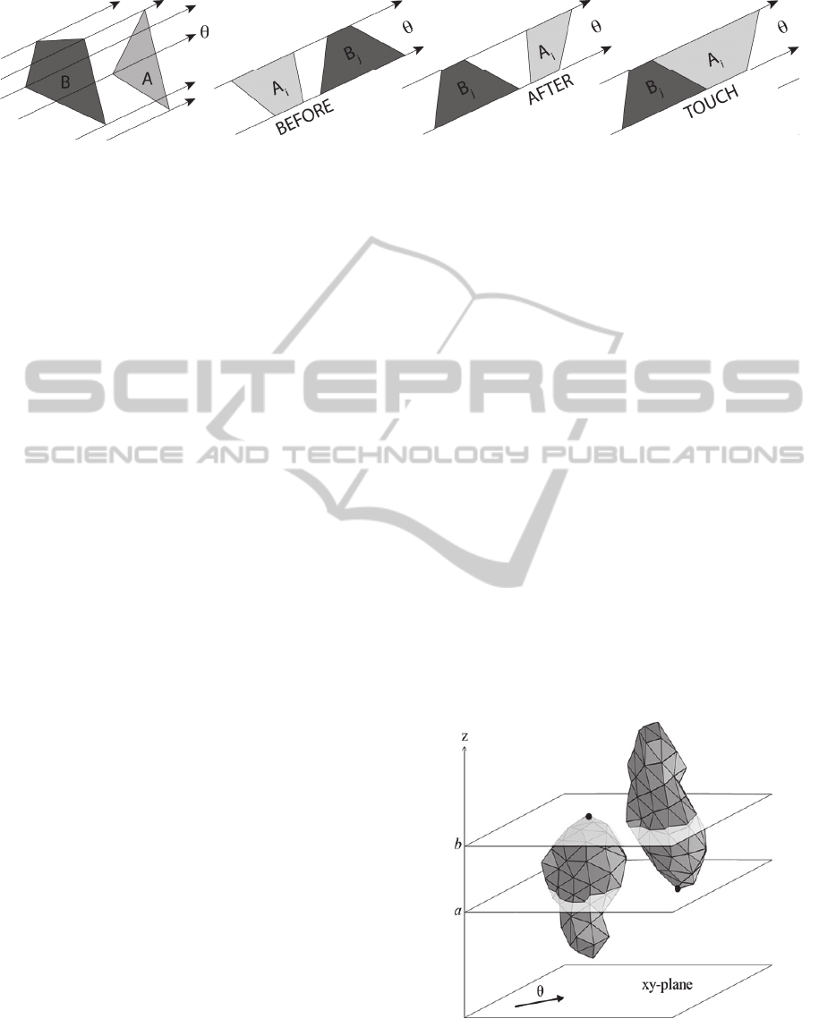
(a) (b) (c) (d)
Figure 2: (a) The objects A and B are broken into trapezoidal (or triangular) pieces A1, A2, etc. and B1, B2, etc. Note that
A and B are not necessarily convex, and there may be more than two pieces between two consecutive lines. Two pieces Ai
and Bj between the same two consecutive lines can be arranged in three possible ways: (b), (c) or (d). Note that in (b), the
trapezoids may share one vertex or one edge; in (c) they may only share one vertex.
2.3 Reference Directions
Practically, of course, only a finite number of direc-
tions can be considered when calculating a force
histogram. An important issue is the choice of these
reference directions. The higher the number of re-
ference directions, the more complete the collected
histogram data, but the longer the processing time.
In the 2D case, the reference directions are usu-
ally chosen so that they are evenly distributed in
space (Matsakis et al., 2011). Since a direction  can
be represented by a point p on the unit circle centred
at the origin  (choose p such that p=), the prob-
lem comes down to finding an even distribution of
points on the circle. The set of reference directions
therefore corresponds to the set of vertices of a
regular convex polygon.
In the 3D case, the unit circle becomes the unit
sphere and regular convex polygons become regular
convex polyhedra. There are only five such poly-
hedra (known as the Platonic solids). One must thus
reflect on what an even distribution of an arbitrary
number of points on a sphere is. The topic has at-
tracted the attention of a wide variety of researchers
(Saff and Kuijlaars, 1997) (Darvas, 2007), and many
different criteria for point distribution can be found
in the literature. The general idea is to optimize
some function of the positions of the points on the
sphere. As an example, one may want to see the
points as electrons that repel each other with a force
given by Coulomb's law and determine the mini-
mum energy configuration. This is the Thomson
problem (Thomson, 1904). Practically, points are
first randomly generated on the sphere, and then an
iterative process allows a stable configuration to be
found. For example, Bourke uses hill climbing
(Bourke, 1996), while Semechko uses a more effi-
cient adaptive Gauss-Seidel update scheme (Se-
mechko, 2012).
3 ALGORITHM
The calculation of a force histogram that represents
the relative position of two 3D connected objects in
vector form is described, in pseudocode, on the next
page. It relies on a simple numerical integration
technique called the composite midpoint rule. The
integral of a function f over an interval [a,b] is cal-
culated as follows: [a,b] is divided into subintervals
of equal length; the integral of f over each subinter-
val [a
i
,a
i+1
] is approximated by (a
i+1
a
i
)
f((a
i
+a
i+1
)/2); the integral of f over [a,b] is obtained
by adding up all the results. In our algorithm, each
force histogram value h() is approximated using
this technique (hence the for loop; line 13). First, the
direction  is rotated together with the objects so
that it lies in the xy-plane (line 14; Fig. 3). The
domain of integration [a,b] can then be easily
determined by sorting the vertices along the z-axis
(line 15; Fig. 3).
Figure 3: Each plane parallel to the xy-plane and with z-
coordinates between a and b slices the 3D objects into 2D
objects. The force in direction  between the 3D objects is
the integral over [a,b] of the force in direction  between
the 2D objects.
ICPRAM2014-InternationalConferenceonPatternRecognitionApplicationsandMethods
106

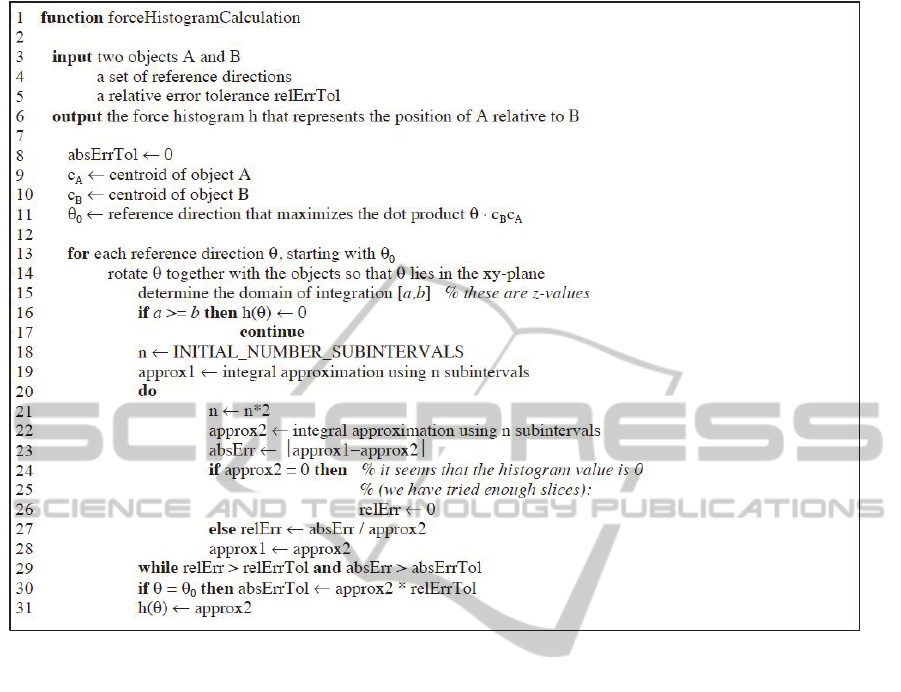
Each plane parallel to the xy-plane and with z-
coordinates between a and b slices the two 3D
vector objects into two 2D vector objects (which
may have multiple connected components). h() is
the integral over [a,b] of the force in direction 
between these 2D objects (a force calculated as in
Section 2.2). The number of subintervals considered
is first set to INITIAL_NUMBER_ SUBINTERVALS
(line 18). This number is then repeatedly doubled
(line 21) until the approximation of the integral is
found satisfactory (line 29). The accuracy of nu-
merical integration is controlled by the relative and
absolute error tolerances relErrTol and absErrTol
(line 29). The absolute difference between two con-
secutive approximations is used as an estimate of the
absolute error absErr (line 23). An estimate of the
relative error relErr follows (line 27). The reference
direction 
0
closest to the direction defined by the
centroids of the objects (lines 9-11) is likely to give
one of the highest force histogram values. It is
therefore considered first (line 13) and used to de-
termine absErrTol (line 30). The combined use of
relErrTol and absErrTol (line 29) stems from the
following: assume the relative error tolerance in
input (line 5) is 1% and the true force histogram
values in some directions 
1
and 
2
are 100 and 10;
if we accept 99 as an approximation of the first
value (relative error 1%, absolute error 1), we should
accept 9 as an approximation of the second value
(relative error 10%, absolute error 1).
4 EXPERIMENTS
The experimental setup is described in Section 4.1
and the results are given and discussed in Section 4.2.
4.1 Setup
The algorithm for force histogram calculation in the
case of 3D vector objects was implemented in C.
The experiments were conducted on a machine run-
ning the Linux 3.11.1 kernel with the AMD Phenom
II X6 1055T processor, 2.8GHz, 8 GB. They involve
the five objects A, B, C, D and T shown in Fig. 4.
The scene is relatively simple, but it is a familiar
scene, with common real-world objects, and ap-
proximating each object by its centre or minimum
bounding box would be doomed to failure.
AFirstAlgorithmtoCalculateForceHistogramsintheCaseof3DVectorObjects
107

Three sets of reference directions are used for
force histogram calculation: one with 102 directions
(neighbour directions are about 20 apart), one with
414 directions (10 apart), and one with 1646 direc-
tions (5 apart). Each set of reference directions is a
set of evenly distributed directions that includes the
set {above, below, left, right, front, behind} of
cardinal directions. See Fig. 5.
Assume h
1
and h
2
are two force histograms cal-
culated using the same set of reference directions.
How to compare these histograms? In (Matsakis et
al., 2004), over twenty similarity measures are
examined for the comparison of 2D force histo-
grams, and two are retained: the Tversky index
min(h
1
(),


h
2
())
max(h
1
(),


h
2
())
(4)
and the Pappis’ measure
1 
h
1
()  h
2
()


h
1
()  h
2
()


(5)
Both can be applied to 3D histograms as well, and
they are used in Section 4.2.
A force histogram associated with two 2D ob-
jects A and B allows various spatial relationships
between these objects to be assessed. In particular,
the histogram can be used to calculate the truth value
of a proposition such as “A is in direction  of B
”
(e.g., “A is to the right of B
”, “A is above B ”). Dif-
ferent methods can actually be applied (Matsakis et
al., 2011). Those considered in Section 4.2 are the
aggregation and effective force methods, as they can
easily be extended to the handling of 3D histograms.
Finally, note that the relative error tolerance
relErrTol (Section 3) may take three different values
in Section 4.2: 0.1 (10%), 0.01 (1%), or 0.001
(0.1%). Moreover, the constant INITIAL_NUMBER_
SUBINTERVALS is set to 2.
4.2 Results
A force histogram h associated with a pair of 3D
objects can be graphically represented by the surface
Figure 4: The objects: 1 table (48 vertices) and 4 chairs (128 vertices each).
(a) (b) (c)
Figure 5: (a) The set of 102 reference directions. (b) 414 reference directions. (c) 1646 reference directions.
chair C
chair A
chair B
chair D
table T
ICPRAM2014-InternationalConferenceonPatternRecognitionApplicationsandMethods
108

(h()+R), where the constant R is a positive real
number and the variable  is a direction (i.e., a unit
vector). This surface is wrapped around the sphere
of radius R, and bumps on it indicate the presence of
forces. See Fig. 6.
Table 1 reports the truth values in the cardinal di-
rections for each object pair. We believe the reader
will find these values consistent with their own per-
ception of the scene. 0 means “totally false” while 1
means “totally true”. According to the aggregation
method, an object may be, to some extent, simulta-
neously above and belowor to the left and to the
right, front and behindanother one. The effective
force method disagrees with this point of view, and
has more clear-cut opinions. These are the main
differences between the two methods.
Not surprisingly, the processing times increase
when the relative error tolerance decreases (Table
2a). On average, rotating the objects and determin-
ing a domain of integration are procedures that take
about 0.0001 second each (Table 2b), i.e., only 2%
(resp. 1%, 0.2%) of the time needed to calculate a
force histogram value when relErrTol is 10% (resp.
1%, 0.1%). See the numbers in bold in Table 2ab
(0.0001/0.00542%, 0.0001/0.01371%, etc.). Cal-
culating a 2D force is as fast, but the procedure is
repeated many times. In the end, it represents about
11% (resp. 15%, 15%) of the time needed to calcu-
late a force histogram value when relErrTol is 10%
(resp. 1%, 0.1%). See the numbers in bold in Table
2ac (60.0001/0.005411%, 200.0001/0.013715%,
etc.). Slicing the objects is by far the most time con-
suming. Overall, it represents about 55% (resp. 73%,
75%) of the time needed to calculate a force histo-
gram value when relErrTol is 10% (resp. 1%, 0.1%).
See the numbers in bold in Table 2ac (6
0.0005/0.005456%, 200.0005/0.013773%, etc.).
The relative error tolerance has a visible impact
on the force histogram. See Fig. 7. However, in
applications where histograms are calculated only to
be compared with each other, setting relErrTol to
0.01 seems to be a good choice. Indeed, a histogram
calculated with relErrTol = 0.01 is obtained much
faster than and is very similar (a 98% to 99% simi-
larity, as shown in Table 3) to the histogram calcu-
lated with relErrTol = 0.001. In applications where
truth values are extracted from force histograms,
relErrTol = 0.1 might be enough when using the
aggregation method, since relErrTol = 0.001 only
gives a 1% absolute difference in truth value (at
worst). See Table 4. When using the effective force
method, relErrTol = 0.1 (resp. 0.01) vs. relErrTol =
0.001 gives a less than 1% absolute difference in
truth value, on average, but that difference may
reach 17% (resp. 9%) in the worst case. The number
of reference directions seems to have even a bigger
impact on truth values than the relative error
tolerance. When using the aggregation method (resp.
effective force method), 414 vs. 1646 directions
gives a less than 1% absolute difference in truth
value, on average, but that difference may reach 5%
(resp. 13%) in the worst case. See Table 5.
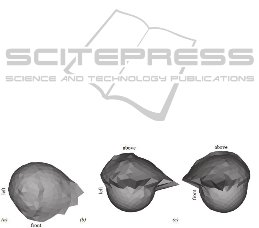
Figure 6: Three different views of the same force histogram: (a) from above, (b) from front, (c) from right. The histogram
represents the position of the chair C relative to the table T. It has been calculated using 414 reference directions and a
relative error tolerance of 1%.
AFirstAlgorithmtoCalculateForceHistogramsintheCaseof3DVectorObjects
109

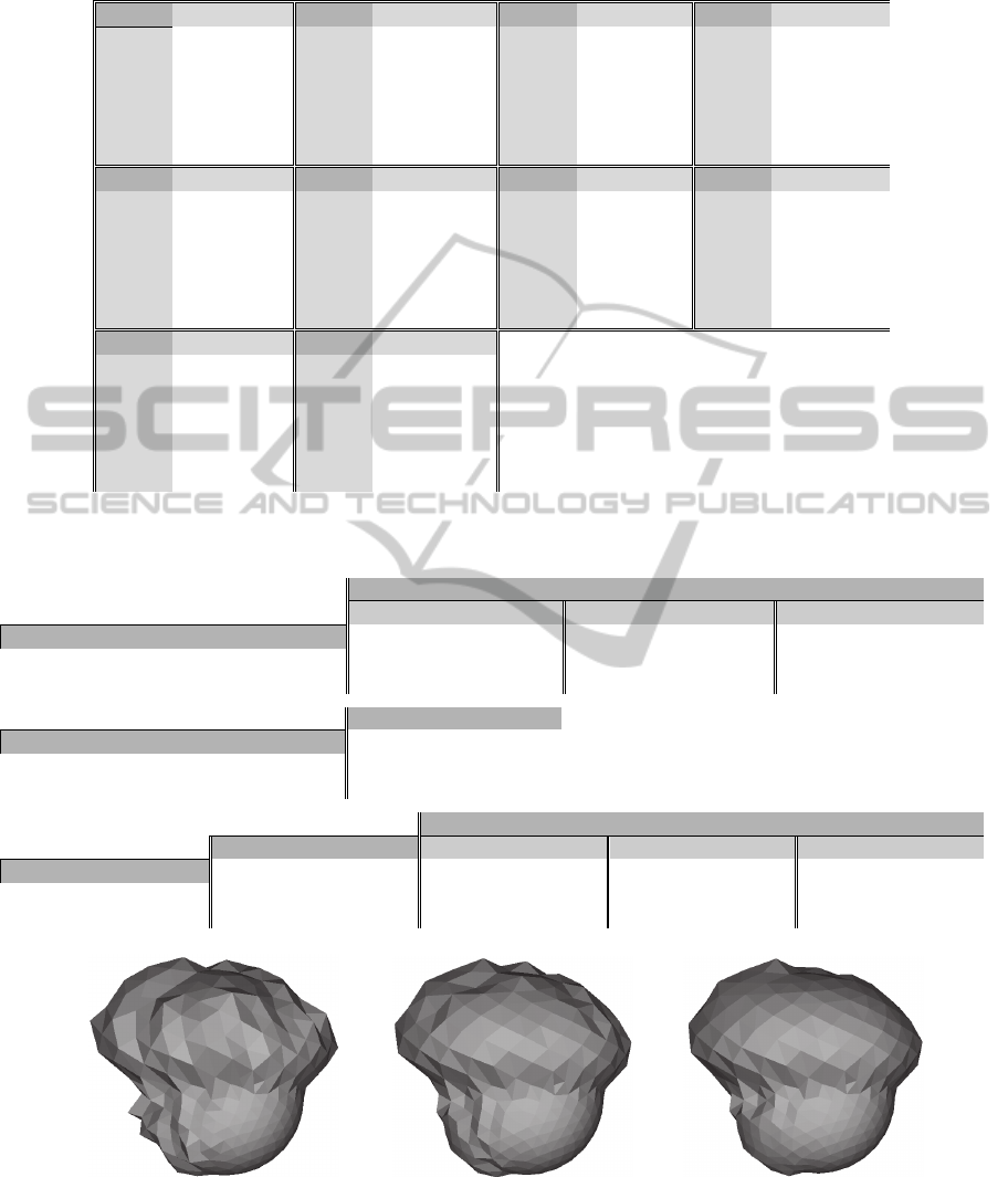
Table 1: The truth values in the cardinal directions for each object pair in the scene. These values are extracted from the
force histograms (414 directions, 1% relative error tolerance) using the aggregation and effective force methods.
B / A
agg eff
C / B
agg eff
A / T
agg eff
C / T
agg eff
above
below
left
right
front
behind
0.44
0.02
0.14
0.16
0.12
0.22
0.86
0
0
0.06
0
0.17
above
below
left
right
front
behind
0.13
0.00
0.48
0
0
0.48
0.46
0
0.75
0
0
0.72
above
below
left
right
front
behind
0.03
0.19
0.15
0.17
0.57
0
0
0.40
0
0.02
0.84
0
above
below
left
right
front
behind
0.37
0.01
0.21
0.15
0.10
0.26
0.84
0
0.06
0
0
0.24
C / A
agg eff
D / B
agg eff
B / T
agg eff
D / T
agg eff
above
below
left
right
front
behind
0.17
0.00
0.40
0
0
0.55
0.47
0
0.65
0
0
0.74
above
below
left
right
front
behind
0.02
0.08
0.08
0.03
0
0.83
0
0.38
0.23
0
0
0.92
above
below
left
right
front
behind
0.05
0.15
0.16
0.17
0.56
0
0
0.30
0
0.06
0.85
0
above
below
left
right
front
behind
0.04
0.37
0.18
0.21
0.05
0.24
0
0.57
0
0.05
0
0.36
D / A
agg eff
D / C
agg eff
0.02
0.02
0.02
0.02
0
0.94
0
0
0
0
0
1.00
0.00
0.24
0
0.72
0.05
0.04
0
0.51
0
0.85
0.17
0
Table 2: Processing times (in seconds). The force histograms are calculated for every pair of objects in the scene, using 414
reference directions.
Processing time
(a) relErrTol = 0.1 relErrTol = 0.01 relErrTol = 0.001
procedure min ave max min ave max min ave max
calculating a force histogram 1s 2s 4s 1s 6s 14s 2s 24s 86s
calculating a force histogram value 0.0007
0.0054
0.0935 0.0007
0.0137
0.7628 0.0007
0.0574
3.5135
(b) processing time
procedure min ave max
rotating the objects 0.0001
0.0001
0.0004
determining a domain of integration 0.0001
0.0001
0.0001
number of times the procedure is applied (per direction)
(c) processing time relErrTol = 0.1 relErrTol = 0.01 relErrTol = 0.001
procedure min ave max min ave max min ave max min ave max
slicing the objects 0.0003
0.0005
0.0009
0
6
126 0
20
1022 0
86
4094
calculating a 2D force 0.0000
0.0001
0.0014
(a) (b) (c)
Figure 7: These force histograms, which are shown from the same point of view, represent the position of the chair A
relative to the chair B. They have been calculated using 414 reference directions and a relative error tolerance of (a) 10%
(b) 1% (c) 0.1%.
above
front
ICPRAM2014-InternationalConferenceonPatternRecognitionApplicationsandMethods
110

Table 3: Comparing force histograms. For every pair of objects in the scene, compare the force histograms calculated using
414 reference directions and two different relative error tolerances.
similarity
Tversky index Pappis’ measure
relative error tolerance min ave max min ave max
0.1 vs. 0.01 0.84 0.92 0.97 0.91 0.96 0.98
0.1 vs. 0.001 0.84 0.91 0.96 0.91 0.95 0.98
0.01 vs. 0.001 0.97
0.98
0.99 0.99
0.99
1.00
Table 4: Comparing truth values (I). For every pair of objects in the scene, calculate the force histograms using 414
reference directions and two different relative error tolerances; then, compare the truth values obtained in every reference
direction.
absolute difference
aggregation method effective force method
relative error tolerance min ave max min ave max
0.1 vs. 0.01 0 0.002 0.013 0 0.005 0.169
0.1 vs. 0.001 0 0.002
0.012
0 0.005
0.169
0.01 vs. 0.001 0 0.001 0.004 0 0.002
0.086
Table 5: Comparing truth values (II). For every pair of objects in the scene, calculate the force histograms using a relative
error tolerance of 0.01 and two different sets of reference directions; then, compare the truth values obtained in every
cardinal direction (above, below, left, right, front, behind).
absolute difference
aggregation method effective force method
number of directions min ave max min ave max
102 vs. 414 0 0.012 0.063 0 0.025 0.195
102 vs. 1646 0 0.014 0.093 0 0.029 0.280
414 vs. 1646 0
0.005 0.054
0
0.009 0.134
5 CONCLUSIONS
We have presented in this paper the first algorithm
for quantitative relative position descriptor calcu-
lation in the case of 3D objects in vector form. We
have built on the histogram of forces because its
mathematical definition holds in any Euclidean
space and theory endows it with remarkable proper-
ties. A force histogram associated with 2D objects
allows various spatial relationships between these
objects to be assessed through the calculation of
truth values; we have shown that the same holds for
a force histogram associated with 3D objects, and
we have shown that the assessments are consistent
with human perception. The new algorithm is an
approximation algorithm with two parameters: the
set of reference directions and the relative error
tolerance. The higher the number of reference direc-
tions, the more complete the collected histogram
data; the lower the relative error tolerance, the more
accurate the collected data; but the longer the pro-
cessing time. We have provided some insight on
how the two parameters impact the processing times,
the force histograms, and the truth values that can be
extracted from the histograms. In future work, we
will show that the processing times can be drasti-
cally reduced. In particular, we will use a much
more sophisticated numerical integration technique,
and we will calculate special sets of reference direc-
tions that will allow directions to be grouped and
batch processed.
REFERENCES
Bourke, P., 1996. Distributing Points on a Sphere. Avail-
able: http://paulbourke.net/geometry/circlesphere/. Last
accessed 23rd Aug 2013.
Darvas, G., 2007. From Viruses to Fullerene Molecules. In
Darvas, G. (Author): Symmetry: Cultural, Historical
and Ontological Aspects of Science Arts Relations; the
Natural and Man-Made World in an Interdisciplinary
Approach, Springer, 215-41.
Kwasnicka, H., Paradowski, M., 2005. Spread Histogram
— A Method for Calculating Spatial Relations Between
Objects. In Proceedings of the 4th Int. Conf. on Com-
puter Recognition Systems (CORES), 249-56.
Matsakis, P., Keller, J., Sjahputera, O., Marjamaa, J., 2004.
The Use of Force Histograms for Affine Invariant
Relative Position Description. In IEEE Trans. on Pat
AFirstAlgorithmtoCalculateForceHistogramsintheCaseof3DVectorObjects
111

tern Analysis and Machine Intelligence, 26(1):1-18.
Matsakis, P., Wendling, L., Ni, J., 2011. A General
Approach to the Fuzzy Modeling of Spatial Rela-
tionships. In Jeansoulin, R., Papini, O., Prade, H.,
Schockaert, S. (Eds.): Methods for Handling Imperfect
Spatial Information, Springer-Verlag, 49-74.
Miyajima, K., Ralescu, A., 1994. Spatial Organization in
2D Images. In Proceedings of the 3rd Int. Conf. on
Fuzzy Systems (FUZZ’IEEE), 1:100-5.
Recoskie, D., Xu, T., Matsakis, P., 2012. A General
Algorithm for Calculating Force Histograms Using
Vector Data. In Proceedings of the 1st Int. Conf. on
Pattern Recognition Applications and Methods
(ICPRAM), 86-92.
Saff, E., Kuijlaars, A., 1997. Distributing Many Points on a
Sphere. In The Mathematical Intelligencer, 19:5–11.
Semechko, A., 2012. Uniform Sampling of a Sphere. Avail-
able: www.mathworks.com/matlabcentral/fileexchange/
37004-uniform-sampling-of-a-sphere/. Last accessed
23rd Aug 2013.
Shyu, C. R., Klaric, M., Scott, G. J., Barb, A. S., Davis, C.
H., Palaniappan, K., 2007. GeoIRIS: Geospatial In-
formation Retrieval and Indexing System—Content
Mining, Semantics Modeling, and Complex Queries.
In IEEE Trans. on Geoscience and Remote Sensing,
45(4):839-52.
Sjahputera, O., Keller, J. M., 2007. Scene Matching Using
F-Histogram-Based Features with Possibilistic C-
Means Optimization. In Fuzzy Sets and Systems,
158(3):253-69.
Skubic, M., Perzanowski, D., Blisard, S., Schultz, A.,
Adams, W., Bugajska, M., Brock, D., 2004. Spatial
Language for Human-Robot Dialogs. In IEEE Trans. on
Systems, Man, and Cybernetics Part C, 34(2): 154-
67.
Thomson, J., 1904. On the structure of the atom: an investi-
gation of the stability and periods of oscillation of a
number of corpuscles arranged at equal intervals around
the circumference of a circle; with application of the re-
sults to the theory of atomic structure. In Philosophical
Magazine, 7(39):237–65.
Vaduva, C., Faur, D., Gavat, I., 2010. Data Mining and
Spatial Reasoning for Satellite Image Characterization.
In Proceedings of the 8th Int. Conf. on Communica-
tions (COMM), 173-76.
Wang, Y., Makedon, F., 2003. R-Histogram: Quantitative
Representation of Spatial Relations for Similarity-Based
Image Retrieval. In Proceedings of the 11th Int. Conf.
on Multimedia (MULTIMEDIA), 323-6.
Zhang, K., Wang, K.-P., Wang, X.-J., Zhong, Y.-X., 2010.
Spatial Relations Modeling Based on Visual Area His-
togram. In Proceedings of the 11th Int. Conf. on Soft-
ware Engineering Artificial Intelligence Networking
and Parallel/Distributed Computing (SNPD), 97-101.
ICPRAM2014-InternationalConferenceonPatternRecognitionApplicationsandMethods
112