Classical Dynamic Controllability Revisited
A Tighter Bound on the Classical Algorithm
Mikael Nilsson, Jonas Kvarnstr¨om and Patrick Doherty
Department of Computer and Information Science, Link¨oping University, SE-58183 Link¨oping, Sweden
Keywords:
Temporal Networks, Dynamic Controllability.
Abstract:
Simple Temporal Networks with Uncertainty (STNUs) allow the representation of temporal problems where
some durations are uncontrollable (determined by nature), as is often the case for actions in planning. It is es-
sential to verify that such networks are dynamically controllable (DC) – executable regardless of the outcomes
of uncontrollable durations – and to convert them to an executable form. We use insights from incremental
DC verification algorithms to re-analyze the original verification algorithm. This algorithm, thought to be
pseudo-polynomial and subsumed by an O(n
5
) algorithm and later an O(n
4
) algorithm, is in fact O(n
4
) given
a small modification. This makes the algorithm attractive once again, given its basis in a less complex and
more intuitive theory. Finally, we discuss a change reducing the amount of work performed by the algorithm.
1 BACKGROUND
Time and concurrency are increasingly considered es-
sential in planning and multi-agent environments, but
temporal representations vary widely in expressiv-
ity. For example, Simple Temporal Problems (STPs,
(Dechter et al., 1991)) allow us to efficiently deter-
mine whether a set of timepoints (events) can be as-
signed real-valued times in a way consistent with a set
of constraints bounding temporal distances between
timepoints. The start and end of an action can be
represented as timepoints, but its possible durations
can only be represented as an STP constraint if the
execution mechanism can choose durations arbitrar-
ily within the given bounds. Usually, exact durations
are instead chosen by nature and agents must generate
plans that work regardless of the eventual outcomes.
STPs with Uncertainty, STPUs (Vidal and Ghal-
lab, 1996), capture this aspect by introducing contin-
gent timepoints that correspond to the end of an ac-
tion, associated with contingent temporal constraints
corresponding to possible durations to be decided by
nature. One must then find a way to assign times
to ordinary controlled timepoints (determine when to
start actions) so that for every possible outcome for
the contingent constraints (action durations), there ex-
ists some solution for the ordinary requirement con-
straints (corresponding to STP constraints).
If an STPU allows us to schedule controlled time-
points (actions to be started) incrementally given that
we receive information when a contingent timepoint
occurs (an action ends), it is dynamically controllable
(DC) and can be efficiently executed by a dispatcher
(Muscettola et al., 1998). Conversely, guaranteeing
that constraints are satisfied when executing a non-
DC plan is impossible, as it would require informa-
tion about future duration outcomes.
Three algorithms for verifying the dynamic con-
trollability of a complete STPU have been published:
1. MMV (Morris et al., 2001), here also called
the classical algorithm. It is a simple algorithm
that derives and tightens constraints using specific
rules. It is easily implemented, captures the intu-
ition behind STNUs and has a direct correctness
proof. Its run-time is pseudo-polynomial.
2. MM (Morris and Muscettola, 2005) builds on the
theory from MMV but uses new, less intuitive
derivation rules. Its run-time complexity is O(n
5
).
3. The Morris algorithm (Morris, 2006) builds on
MM. Its theory and especially analysis contains
several complicated new concepts taking it fur-
ther from the simple intuition of MMV. This is
the fastest algorithm with a complexity of O(n
4
).
In this paper we re-analyze MMV and prove that with
a small modification it is in fact O(n
4
) – the algo-
rithm merely needs to stop earlier. The intuition be-
hind the analysis is that not all of MMV’s derivations
and tightenings are necessary: Only a certain core
of derivations actually matters for verifying dynamic
130
Nilsson M., Kvarnström J. and Doherty P..
Classical Dynamic Controllability Revisited - A Tighter Bound on the Classical Algorithm.
DOI: 10.5220/0004815801300141
In Proceedings of the 6th International Conference on Agents and Artificial Intelligence (ICAART-2014), pages 130-141
ISBN: 978-989-758-015-4
Copyright
c
 2014 SCITEPRESS (Science and Technology Publications, Lda.)

controllability, and when the STNU is DC, this core
is free of cyclic derivations. This can be exploited
through a small change to MMV. Stopping at the right
time also preserves another aspect of MMV: the result
is dispatchable, unlike the result of Morris’ algorithm.
Outline. After providing some fundamental defini-
tions, we describe the MMV algorithm (section 2).
We also present the FastIDC algorithm, which will
provide intuitions for our analysis of MMV (section
3). We compare the derivations made by the two algo-
rithms (section 4) and analyze the length of FastIDC
derivation chains (section 5), resulting in the new al-
gorithm GlobalDC (section 6) which runs in O(n
4
).
GlobalDC is in fact identical to a slightly modified
MMV algorithm.
Definition 1. A Simple Temporal Problem (STP,
(Dechter et al., 1991)) consists of a number of real
variables x
1
, . . . , x
n
and constraints T
ij
= [a
ij
, b
ij
],
i 6= j limiting the temporal distance a
ij
≤ x
j
−x
i
≤ b
ij
between the variables.
We will work with STPs in graph form, with time-
points represented as nodes and constraints as labeled
edges. They are then referred to as Simple Temporal
Networks (STNs). We will also make use of the fact
that any STN can be represented as an equivalent dis-
tance graph (Dechter et al., 1991). Each constraint
[u, v] on an edge AB in an STN is represented as two
corresponding edges in its distance graph: AB with
weight v and BA with weight −u. Computing the all-
pairs-shortest-path (APSP) distances in the distance
graph yields a minimal representation containing the
tightest distance bounds that are implicit in the origi-
nal problem (Dechter et al., 1991). This directly cor-
responds to the tightest interval constraints [u
′
, v
′
] im-
plicit in the original STN.
If the distance graph has a negative cycle, then
no assignment of timepoints to variables satisfies the
STN: It is inconsistent. Otherwise it is consistent
and can be executed: Its events can be assigned time-
points so that all constraints are satisfied. One way of
assigning time-points is using a dispatcher (Muscet-
tola et al., 1998). While a dispatcher may assign any
legal time to an event, in practice one often executes
events as soon as possible given the constraints.
Definition 2. A Simple Temporal Problem with Un-
certainty (STPU) (Vidal and Ghallab, 1996) consists
of a number of real variables x
1
, . . . , x
n
, divided into
two disjoint sets of controlled timepoints R and con-
tingent timepoints C. An STPU also contains a num-
ber of requirement constraints R
ij
= [a
ij
, b
ij
] limiting
the distance a
ij
≤ x
j
− x
i
≤ b
ij
, and a number of con-
tingent constraintsC
ij
= [c
ij
, d
ij
] limiting the distance
c
ij
≤ x
j
− x
i
≤ d
ij
. For the constraints C
ij
we require
[35,40]
[-5,5]
Requirement Constraint
Contingent Constraint
[x,y]
[x,y]
Start
Driving
Wife at
Home
Drive
Start
Cooking
Dinner
Ready
[25,30]
Cook
Wife at
Store
[30,60]
Shopping
Figure 1: Example STNU.
that x
j
∈ C, 0 < c
ij
< d
ij
< ∞.
STPUs in graph form are called STNs with Uncer-
tainty (STNUs). An example is shown in figure 1. In
this example a man wants to cook for his wife. He
does not want her to wait too long after she returns
home, nor does he want the food to wait too long.
These two requirements are captured by a single re-
quirement constraint, whereas the uncontrollable du-
rations of shopping, driving home and cooking are
captured by the contingent constraints. The question
is whether this can be guaranteed regardless of the
outcomes of the uncontrollable durations.
In addition to the types of constraints already ex-
isting in an STNU, some algorithms can also gener-
ate wait constraints that make certain implicit require-
ments explicit for use in further computations.
Definition 3. Given a contingent constraint between
A and B and a requirement constraint from A to C,
the < B,t > annotation on the constraint AC indicates
that execution of the timepointC is not allowed to take
place until after either B has occurred or t units of
time have elapsed since A occurred. This constraint
is called a wait constraint, or wait, between A and C.
As there are events whose occurrence we cannot fully
control, consistency is not sufficient for an STNU to
be executable. However, suppose that for a given
STNU there exists a dynamicexecution strategy that
can assign timepoints to controllable events during
execution, given that at each time, it is known which
contingent events have already occurred. The STNU
is then dynamically controllable (DC) and can be
executed. In figure 1 a dynamic execution strategy
is to start cooking 10 time units after receiving a call
that the wife starts driving home. This guarantees that
cooking is done within the required time, since she
will arrive at home 35 to 40 time units after starting to
drive and the dinner will be ready 35 to 40 time units
after she started driving.
DC STNUs can be executed by a dispatcher tak-
ing uncontrollable events into account. The algorithm
required depends on whether the STNU has been pre-
processed. A dispatcher for STNUs processed by
MMV will be shown later.
ClassicalDynamicControllabilityRevisited-ATighterBoundontheClassicalAlgorithm
131

Algorithm 1: The MMV Algorithm.
Boolean procedure determineDC()
repeat
if not pseudo-controllable then
return false
else
forall the triangles ABC do
tighten ABC using the tightenings in
figure 2
end
until no tightenings were found
return true
2 THE MMV ALGORITHM
Algorithm 1 shows the classical “MMV” algorithm
(Morris et al., 2001) as reformulated and clarified by
(Morris and Muscettola, 2005). Note that these ver-
sions share the same worst case complexity.
The algorithm builds on the concept of pseudo-
controllability (PC), a necessary but not sufficient re-
quirement for dynamic controllability. To test for
pseudo-controllability the STNU is first converted to
an STN by converting all contingent constraints into
requirement constraints. The STN then has to be put
in its minimal representation (see section 1). If the
STN is inconsistent, the corresponding STNU cannot
be consistently executed and is not DC. If the STN
is consistent but a constraint corresponding to a con-
tingent constraint in the STNU became tighter in the
minimal representation, the contingent constraint is
squeezed. Then nature can place the uncontrollable
outcome of the contingent constraint outside what is
allowed by the STN representation, causing execution
to fail. Therefore the STNU is not DC. Conversely, if
the minimal representation is consistent and does not
squeeze any corresponding contingent constraint, the
STNU is pseudo-controllable.
MMV additionally uses STNU-specific tightening
rules, also called derivation rules, which make con-
straints that were previously implicit in the STNU ex-
plicit (figure 2). Each tightening rule can be applied
to a “triangle” of nodes if the constraints and require-
ments of the rule are matched. The result of applying
a tightening is a new or tightened constraint, shown
as bold edges in the leftmost part of the triangle. Note
that unordered reduction generates wait constraints,
which cannot be present in the original STNU.
Algorithm 1 consists of a loop that first verifies PC
and transfers all tighter constraints found by the asso-
ciated APSP calculation to the STNU, then applies all
possible tightenings. For a non-DC STNU, tighten-
ings eventually produce sufficient explicit constraints
Requirement Constraint
Contingent Constraint
Wait Constraint
A
C
B
[x,y]
[u,v]
[y-v,x-u]
Requires: u 0
A
C
B
[x,y]
[u,v]
<B,y-v>
Requires: u < 0 ! v
A
D
C
<B,y>
[u,v]
<B,y-v>
D
[u,v]
<B,y-u>
Requires: y 0, B C
A
C
B
[x,y]
<B,u>
[u,!]
Requires: u ! x Requires: u > x
A
C
<B,y>
[x,y]
[x,y]
<B,y>
Requires: -
A
C
B
[x,y]
<B,u>
[x,!]
Figure 2: Tightenings (derivations) of the MMV algorithm.
for the PC test to detect this (Morris et al., 2001).
The complexity of MMV is said to be O(Un
3
)
where U is a measure of the size of the domain
(the number of constraints and the size of constraint
bounds). This comes from a cost of O(n
3
) per iter-
ation and the fact that each iteration must tighten at
least one constraint leading in the extreme to a neg-
ative cycle. Since the complexity bound depends on
the size of constraint bounds, it is pseudo-polynomial.
If MMV labels an STNU as DC, the processed
STNU can be executed by the dispatcher in algo-
rithm 2,which was originally presented in (Morris
et al., 2001) and is shown here in a different format.
The dispatcher uses two distinct conditions to deter-
mine whether an event e can be executed. First, e
must be enabled, meaning that all events that must be
executed before it have actually been executed. These
events can be found through the outgoing negative re-
quirement edges. Second, e must be live, meaning
that it is within its permitted time window. These
time windows are related to the constraints from the
original STNU and cannot be determined in advance.
Instead they are initialized to [0, ∞] and then dynam-
ically updated as events actually occur during execu-
tion. Observations of uncontrollable events are han-
dled through the same mechanism, causing the time
windows of “dependent” nodes to be updated. When
an event becomes enabled, its time window is guar-
anteed to be fully updated. For example, suppose that
Start Cooking in figure 1 is executed at time 50. Then,
and only then, can we infer that Dinner Ready must
occur within the interval [75, 80].
ICAART2014-InternationalConferenceonAgentsandArtificialIntelligence
132

Algorithm 2: STNU Dispatcher.
function DISPATCH( G− STNU )
enabled ← {Temporal-Reference}
executed ← {}
currentTime ← 0
repeat
minTime ← min
e∈enabled
lowerBound(e)
Advance time until uncontrollable event
observed or currentTime = minTime
if uncontrollable event e observed then
execute ← e
Remove any waits conditioned on e
end
else
execute ← any live event in enabled whose
waits are satisfied
end
executed ← executed∪ {execute}
enabled ← enabled\{execute}
Assign currentTime to execute
Propagate execution bounds along constraints to
neighboring events
enabled ← enabled ∪{newly enabled events}
until All nodes are executed
3 THE FASTIDC ALGORITHM
The property of dynamic controllability is “mono-
tonic” in the sense that if an STNU is not DC, it can
never be made DC by further adding or tightening
constraints. Therefore, the non-incremental verifica-
tion performed by MMV is equivalent to starting with
an empty STNU (which is trivially DC) and incre-
mentally adding one edge at a time, verifying at each
step that the STNU remains DC.
We will exploit this fact to compare MMV to the
incremental FastIDC algorithm (Stedl and Williams,
2005; Shah et al., 2007), which will allow us to draw
certain conclusions about MMV. First, though, we
will present and explain FastIDC itself, specifically
its tightening / edge-addition aspect (since loosening
or removing edges will not be required here). As the
original version of this algorithm was incorrect in cer-
tain cases, we use the corrected version shown in al-
gorithm 3 as our starting point (Nilsson et al., 2013).
FastIDC has three main differences compared to
the MMV algorithm.
1: Representation. FastIDC does not work in the
standard STNU representation but uses an extended
distance graph (Stedl, 2004), analogous to the dis-
tance graphs sometimes used for STNs. Requirement
edges and contingent edges are then translated into
pairs of edges of the corresponding type in a manner
similar to what was previously described for STNs.
Algorithm 3: FastIDC – sound version.
function FAST-IDC( G, e
1
, . . . , e
n
)
Q ← sort e
1
, . . . , e
n
by distance to temporal reference
(order important for efficiency, not correctness)
for each modified edge e
i
in ordered Q do
if IS-POS-LOOP( e
i
) then SKIP e
i
if
IS-NEG-LOOP( e
i
) then return false for each
rule (Figure 3) applicable with e
i
as focus do
if edge z
i
in G is modified or created then
Update CCGraph
if Negative cycle created in CCGraph
then return false if G is squeezed then
return false if not
FAST-IDC( G, z
i
)
then
return false
end
end
end
return true
Definition 4. An Extended Distance Graph (EDG)
is a directed multi-graph with weighted edges of
5 kinds: positive requirement, negative requirement,
positive contingent, negative contingent and condi-
tional.
The conditional edges mentioned above, first used by
(Stedl, 2004), are used to represent the waits that can
be derived by MMV. The direction of a conditional
edge is intentionally opposite to that of the wait it en-
codes. This makes the conditional edge more similar
to a negative requirement edge in the same direction,
the difference being the condition.
Definition 5. A conditional edge CA annotated
< B, −w > encodes a conditional constraint: C must
execute after B or at least w time units after A,
whichever comes first. The node B is called the con-
ditioning node of the constraint/edge.
2: Derivation Rules. Partly due to the new represen-
tation, FastIDC uses different derivation rules. These
are shown in EDG form in figure 3, where we have
numbered two rules (D8–D9) that were unnumbered
in the original publication. As we will see later, these
are required for soundness.
3: Traversal Order. FastIDC uses a significantly dif-
ferent graph traversal order. MMV traverses a graph
iteratively, and in each iteration, it considers all “tri-
angles” in a graph in arbitrary order. FastIDC, in con-
trast, uses the concept of focus edges. A focus edge is
an edge that was tightened and may lead to other con-
straints being tightened. FastIDC only applies deriva-
tion rules to focus edges. If this leads to new tightened
edges it will recursively continue to apply the deriva-
tion rules until quiescence. Intuitively, this guarantees
that all possible consequences of any tightening are
covered by the algorithm.
ClassicalDynamicControllabilityRevisited-ATighterBoundontheClassicalAlgorithm
133

A
C
B
v
-x
y
<B,v-y>
A
C
B
v
-x
v-x
A
D
C
<B,-y>
-u
v
<B,u-y>
A
C
B
v
<D,-x>
<D,v-x>
A
D
C
<B,-y>
v
<B,v-y>
A
C
B
-u
-x
y
x-u
A
C
B
-u
y
y-u
B D
A D
Requirement Edge
Contingent Edge
Conditional Edge
Derived Edge – Leftmost
Focus Edge – Topmost (except in D8/D9)
A
C
B
-x
-u
<B,-u>
A
C
B
-x
-x
<B,-u>
u x u > x
Removed Edge
Figure 3: FastIDC derivation rules D1-D9.
FastIDC Details. Being incremental, FastIDC as-
sumes that at some point a dynamically controllable
STNU was already constructed (for example, the
empty STNU is trivially DC). Now one or more re-
quirement edges e
1
, . . . , e
n
have been added or tight-
ened, together with zero or more contingent edges and
zero or more new nodes, resulting in the graph G.
FastIDC should then determine whether G is DC.
The algorithm works in the EDG of the STNU.
First it adds the newly modified or added require-
ment edges to a queue, Q (a contingent edge must be
added before any other constraint is added to its target
node and is then handled implicitly through require-
ment edges). The queue is sorted in order of decreas-
ing distance to the temporal reference (TR), a node
always executed before all other nodes at time zero.
Therefore nodes close to the “end” of the STNU will
be dequeued before nodes closer to the “start”. This
will to some extent prevent duplication of effort by
the algorithm, but is not essential for correctness or
for understanding the derivation process.
In each iteration an edge e
i
is dequeued from Q.
A positive loop (an edge of positive weight from a
node to itself) represents a trivially satisfied constraint
that can be skipped. A negative loop entails that a
node must be executed before itself, which violates
DC and is reported.
If e
i
is not a loop, FastIDC determines whether
one or more of the derivation rules in figure 3 can be
applied with e
i
as focus. The topmost edge in the fig-
ure is the focus in all rules except D8 and D9, where
the focus is the conditional edge < B, −u >. Note that
rule D8 is special: The derived requirement edge rep-
resents a stronger constraint than the conditional fo-
cus edge, so the conditional edge is removed.
For example, consider rule D1. This rule will be
matched if e
i
is a positive requirement edge, there is
a negative contingent edge from its target B to some
other node C, and there is a positive contingent edge
from C to B. Then a new constraint (the bold edge)
can be derived. This constraint is only added to the
EDG if it is strictly tighter than any existing constraint
between the same nodes.
More intuitively, D1 represents the situation
where an action is started at C and ends at B, with
an uncontrollable duration in the interval [x, y]. The
focus edge AB represents the fact that B, the end of
the action, must not occur more than v time units after
A. This can be represented more explicitly with a con-
ditional constraint AC labeled < B, v− y >: If B has
occurred (the action has ended), it is safe to execute
A. If at most v − y time units remain until C (equiv-
alently, at least y− v time units have passed after C),
no more than v time units can remain until B occurs,
so it is also safe to execute A.
Whenever a new edge is created, the corrected
FastIDC tests whether a cycle containing only neg-
ative edges is generated. The test is performed by
keeping the nodes in an incrementally updated topo-
logical order relativeto negativeedges. The unlabeled
graph which is used for keeping the topological order
is called the CCGraph. It contains the same nodes
as the EDG and has an edge between two nodes iff
there is a negative edge between them in the EDG.
See (Nilsson et al., 2013) for further information.
After this a check is done to see if the new edge
squeezes a contingent constraint. Suppose FastIDC
derives a requirement edge BA of weight w, for exam-
ple w = −12, representing the fact that B must occur
at least 12 time units after A. Suppose there is also
a contingent edge BA of weight w
′
> w, for example
w
′
= 10, representing the fact that an action started at
A and ending at B may in fact take as little as 10 time
units to execute. Then there are situations where na-
ture may violate the requirement edge constraint, and
the STNU is not DC.
If the tests are passed and the edge is tighter than
any existing edges in the same position, FastIDC
is called recursively to take care of any derivations
caused by this new edge. Although perhaps not
easy to see at a first glance, all derivations lead to
new edges that are closer to the temporal reference.
Derivations therefore have a direction and will even-
tually stop. When no more derivations can be done
the algorithm returns true to testify that the STNU is
DC. If FastIDC returns true after processing an EDG
ICAART2014-InternationalConferenceonAgentsandArtificialIntelligence
134

B
D
A
C
E
F
5
5
5
<D,-5>
<B,-5>
<F,-5>
10
10
10
-2
-2
-2
Figure 4: Why general reduction is needed.
this EDG can be dispatched directly by the dispatcher
in algorithm 2.
General and Unordered Reductions. In the original
FastIDC presentation the use of unconditional/general
reductions were confounded. As shown here, they are
both needed in their original form.
First, figure 4 shows what happens if FastIDC
(or MMV) would omit general reduction. Suppose
the graph in the figure is built incrementally. When
adding the CB, ED and AF edges, the conditional
edges CA, EC and AE will be derived. FastIDC would
then terminate with a positive verification of DC.
However, the triangle of conditional edges means that
all involved nodes (A/C/E) need to be executed after
each other, an inconsistency which is not discovered.
The edge derived by general reduction is entailed by
the conditional edge and resolves this problem.
Regarding unconditional reduction, suppose the
CB edge in figure 4 had weight 9, giving the CA edge
weight -1. Now C needs to execute 1 time unit after
A or when B is observed. Since B cannot be observed
until at least 2 time units after A the conditional part
of the constraint is of no consequence and a require-
ment edge of weight -1 can be inferred.
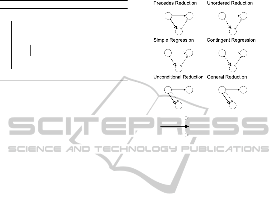
4 COMPARING FASTIDC / MMV
To compare the derivation rules used by MMV to
those of FastIDC, we first need a translation into EDG
format. This is shown in figure 5 where as before the
bold edges are derived. Precedes reduction is split
in two since it adds two edges. Simple regression is
also split in two, one version regressing over a posi-
tive edge and one regressing over a negative edge. All
variables used as weights are considered positive, i.e.,
−u is a negative number (with unconditional reduc-
tion as an exception). The additional requirements
from figure 2 still apply but are omitted for clarity.
Most are encoded by the edge types – for instance in
unordered reduction, only a positive requirementedge
can match the rule, making the v > 0 requirement im-
plicit. We now see the following similarities:
• Precedes Reduction 1 (PR1) is identical to D6.
Precedes Reduction 1 & 2
A
C
B
-u
-x
x-u
A
C
B
v
y
v-y
Unordered Reduction
A
C
B
v
y
<B,v-y>
Simple Regression 1 & 2
A
D
C
<B,-y>
v
<B,v-y>
Contingent Regression
A
D
C
<B,-y>
<B,u-y>
Unconditional
Reduction
A
C
B
-x
-u
<B,-u>
General
Reduction
A
C
B
-x
-x
<B,-u>
y
-x -x
v
-u
A
D
C
<B,-y>
<B,-v-y>
-v
Requirement
Contingent
Conditional
Figure 5: Classical derivations in EDG format.
• Unordered reduction is equivalent to D1. How-
ever without the extra requirement (u ≥ 0) used by
MMV to distinguish between applying PR2 and
unordered reduction, FastIDC will always apply
unordered reduction, even when MMV instead
would apply PR2. It can be shown that if the sit-
uation calls for an application of PR2, FastIDC
derives the same edge as MMV through conver-
sion of the conditional edge resulting from D1
into a requirement edge (via unconditional reduc-
tion, D8). If the application of PR2 directly leads
to non-DC detection, FastIDC also detects this di-
rectly. So PR and unordered reduction are handled
by D1, D6 and D8 together.
• Simple regression 1 is equivalent to D3 and D5.
The only difference between D3 and D5 is which
edge is regarded as focus.
• Contingent regression is identical to D2.
• Unconditional Reduction is identical to D8.
• General Reduction is identical to D9.
Thus, the only significant differences are:
• FastIDC derivations has no counterpart to Simple
Regression 2.
• D4 and D7 have no counterpart rules in MMV.
These derive shortest path distances towards ear-
lier nodes in the STNU. This derivation is present
and handled by the APSP calculation in MMV.
We see that MMV does everything that the FastIDC
derivations do, and also applies SR2 and a complete
APSP calculation.
It can in fact be seen that SR2 is not needed, not even
by MMV. Figure 6 shows the situation where a con-
ditional edge CA is regressed over an incoming neg-
ative requirement edge DC. Adding a constraint DA
ClassicalDynamicControllabilityRevisited-ATighterBoundontheClassicalAlgorithm
135

A
D
C
-v
<B,-y>
<B,-v-y>
Figure 6: Simple regression when the edge is negative.
to ”bridge” two consecutive negative edges is always
redundant both for execution and for DC verification.
From an execution perspectivethis is easily seen since
C is always executed before D which ensures that the
chain of constraints is respected without the addition
of DA. From a verification perspective this can be
seen since the derived constraint is in fact weaker than
the two original constraints. If B is executed before C
the DA constraint ”forgets” about the −v constraint
which must still be fulfilled. So the original two con-
straints are not only sufficient to guarantee the DA
constraint, they are tighter and so the DA constraint
can be skipped.
FastIDC Correctness. Nilsson (2013) includes a
brief correctness sketch for the modified FastIDC al-
gorithm. Since our MMV analysis depends on this,
we now expand upon the sketch.
FastIDC cannot derive stronger constraints than
MMV does. Since MMV applies its derivations and
shortest-path calculations to all triangles of nodes un-
til quiescence, the recursive traversal performed by
FastIDC clearly cannot process a focus edge that
MMV does not process. Further, every derivation rule
applied by FastIDC is also used by MMV: D4 and D7
are implicitly performed through APSP calculations,
while the other rules are directly applied.
Case 1. FastIDC indicates that the STNU is not DC.
Then applying the derivation rules has resulted in the
detection of a negative cycle or a local squeeze. The
constraints generated by MMV would be at least as
strong and would therefore also result in a negative
cycle or local squeeze. The pseudo-controllabilitytest
used by MMV would detect this, signalling that the
STNU is notDC. Since MMV is correct, FastIDC was
also correct in this case.
Case 2. FastIDC indicates that the STNU is DC. We
will show that it is dispatchable by the dispatcher in
algorithm 2, which in turn entails that there must exist
a dynamic execution strategy (the one applied by the
dispatcher). Thus, the STNU is DC and FastIDC is
correct.
Proving this requires some knowledge of the dis-
patcher (algorithm 2). When the dispatcher exe-
cutes or observes the execution of a node, execution
bounds are propagated to all neighboring nodes. Up-
per bounds are propagated along positive edges, while
lower bounds are propagated “backwards” along neg-
ative edges, which includes all conditional edges.
To unify the cases in the following discussion we
assume that when an uncontrollable event is observed,
a time window for the event is propagated to it con-
taining only the observed time. This approach lets
us compare propagatedbounds from both controllable
and uncontrollable nodes.
Now, let H be a DC STNU constructed
through repeated applications of FastIDC. Add
one or more edges e
1
, . . . , e
n
, and assume that
FastIDC(G,e
1
, . . . , e
n
) classifies G as DC. We then
know that:
1. It does not contain a cycle consisting only of neg-
ative requirement edges, as this would have been
detected by the CCGraph (Nilsson et al., 2013).
2. It does not contain a cycle consisting only of neg-
ative requirement edges and conditional edges,
since general reduction (D9) would have created
a cycle of negative requirement edges from this.
Therefore it is not possible for the dispatcher to end
up in a deadlock where no nodes are executable. But
theoretically there could be some combined outcomes
of the uncontrollable events for which execution will
fail because the propagation of execution bounds re-
sults in an empty time window for some event.
Assume that this happens: At least one node re-
ceives an empty time window. Let X be the first node
for which this happens during the propagation pro-
cedure. The time window was initially [0, ∞], and
must have been intersected with at least two propa-
gated time windows that do not overlap, so that the
upper bound of X is below its lower bound. The up-
per bound and lower bound must then be caused by
propagation from distinct nodes. Thus we have a tri-
angle AXB in the EDG where an incoming edge AX
has constrained the upper bound of X and an outgoing
edge XB has constrained the lower bound of X.
We will now consider all possible edge types for
these incoming and outgoing edges and show that in
each case, FastIDC would in fact have derived an ad-
ditional constraint ensuring that the time window for
X could not have become empty. First, suppose the
upper bound for X was propagated from a contingent
constraint AX. The lower bound might then have orig-
inated in:
1. A negative requirement edge XB. Then rule D6
would have generated a constraint AB constrain-
ing the relative timing between the execution of
A and that of B. This constraint would have pre-
vented the intervals propagated from A and B to X
from having an empty intersection.
2. A conditional edge XB, in which case X would be
ICAART2014-InternationalConferenceonAgentsandArtificialIntelligence
136

Table 1: The derived edges compared to the focus edges.
Rule Effect
D1 The target of the derived edge is an earlier node.
D2,D6 The source of the derived edge is an earlier node.
D3,D7 The source of the derived edge is an earlier or
unordered node.
D4,D5 The target of the derived edge is an earlier node.
D8,D9 The derived edge connects the same nodes.
“protected” in a similar way by a constraint gen-
erated by D2.
Second, suppose that the upper bound for X was prop-
agated from a positive requirement edge AX. The
lower bound might have originated in:
1. A negative requirement edge XB: X protected by
D4 or D7.
2. A conditional edge XB: X protected by D3 or D5.
3. A contingent constraint XB: X protected by D1.
Note that we treat contingent edges as a whole con-
straint since they collapse the interval to a point and
as such it does not matter if the positive or negative
edge is considered as propagating the time value.
Thus, for X to receive an empty time window, A
or B (or both) must also have received an empty time
window from the propagation of AB together with the
other constraints in the EDG. Furthermore, since they
propagated constraints to X, they must have been dis-
patched before X. This contradicts the assumption
that X was the first node to receive an empty time
window. Since no additional assumptions were made
about X, no node can receive an empty time window
during dispatch. The dispatcher together with the pro-
cessed STNU therefore constitute a dynamic execu-
tion strategy, and the STNU is DC.
5 FOCUS PROPAGATION
If we apply rules D1–D9 in figure 3, every derived
edge has a uniquely defined “parent”: The focus edge
of the derivation rule. Unless this edge was already
present in the original graph, it (recursively) also has
a parent. This leads to the following definition.
Definition 6. Edges that are derived through figure-3
derivations are part of a derived chain, where the
parent of each edge is the focus edge used to derive it.
We observe the following:
• A contingent constraint orders the nodes it con-
strains. In EDG form we see this by the fact that
the target of a negative contingent edge is always
executed before its source.
• Either D8 or D9 is applicable to any conditional
edge. Thus there will always be an order between
its nodes set by the negative requirement edge
from D8/D9: The target node of a conditional
constraint is always executed before its source.
This leads directly to the facts in table 1. Here, node
n
1
is considered earlier than n
2
if n
1
must be executed
before n
2
in every dynamic execution strategy and for
all duration outcomes. Similarly, node n
1
is consid-
ered unordered relative to n
2
if their order can differ
depending on strategy or outcome.
We now consider the structure of derived chains
in DC STNUs. The focus will be on the direction and
weight of each derived edge, ignoring whether edges
are negative, positive, requirement or conditional (but
still keeping track of contingent edges).
Lemma 1. Suppose all rules in figure 3 are applied
to the EDG of a dynamically controllable STNU until
no more rules are applicable. Then, all derived chains
are acyclic: No derivation rule has generated an edge
having the same source and target as an ancestor of
its parent edge along the current chain.
Proof. Note that by the definition of acyclicity we al-
low “cycles” of length 1. These can only be created
by applications of D8–D9 in a DC STNU.
For D1–D7, each derived edge shares one node
with its parent focus edge, but has another source or
target. We can then track how the source and target of
the focus edge changes through the chain.
Table 1 shows that only derivation rules D1, D4
or D5 result in a different target for the derived edge
compared to the focus edge. The new target has al-
ways “moved” along a negativeedge, so it must be ex-
ecuted earlier than the target of the focus edge. Since
the STNU is DC, its associated STN cannot have neg-
ative cycles. Thus, if the target changes along a chain,
it cannot “cycle back” to a previously visited target.
Rules D2, D3, D6 and D7 result in a different
source for the derived edge. This source may be ear-
lier or later than the source of the focus edge, so these
rules can be applied in a sequence where the source of
the focus edge “leaves” a node n and eventually “re-
turns”. Suppose that this happens and the target n
′
has
not changed. This must occur through applications of
rules D2, D3, and/or D6–D9. No such derivation step
decreases the weight of the focus edge. Therefore,
when the source returns to n, the new edge to be de-
rived between n and n
′
cannot be tighter than the one
that already exists. No new edge is actually derived.
Thus, if the source changes along a chain, it cannot
“cycle back” to a previously visited source.
This fact together with the previous lemma limits the
ClassicalDynamicControllabilityRevisited-ATighterBoundontheClassicalAlgorithm
137

Figure 7: Situation where D2 or D6 is applied.
length of a derived chain to 2n
2
since we have at
most n
2
distinct ordered source/target pairs and can
at most have one application of D8/D9 inbetween
source/target movements. The use of chains to reach
an upper bound on iterations is inspired by (Mor-
ris and Muscettola, 2005) where an upper bound of
O(n
5
) is reached for MM.
Note that FastIDC derivations together with local
consistency checks and global cycle detection is
sufficient to guarantee that all implicit constraints
represented by a chain of negative edges are re-
spected, or non-DC is reported. There is no need to
add these implicit constraints but the next proof will
make use of the fact that they exist.
Some derivations carried out by FastIDC can be
proven not to affect the DC verification process, and
hence we would like to avoid doing these. These can
both be derivations of weaker constraints and con-
straints that are implicitly checked even if they are
not explicitly present in the EDG. In order to single
out the needed derivations we define critical chains.
Definition 7. A critical chain is a derived chain in
which all derivations are needed to correctly classify
the STNU. If any derivation in the chain was missing,
a non-DC STNU might be misclassified as DC.
Given a focus edge, one or more derivations may
be applicable. Those that would extend the current
critical chain into a non-critical one can be skipped
without affecting classification. We therefore identify
some criteria that are satisfied in all critical chains.
Theorem 1. Given a DC STNU:
1. A D1 derivation for a specific contingent con-
straint C can only be part of a critical chain once.
2. At most one derivation of type D2 and D6 involv-
ing a specific contingent constraint C can be part
of a critical chain.
Proof sketch: Part 1 is shown as in the proof of
lemma 1: The target cannot come back for another
D1 application to the same contingent node.
We use figure 7 to illustrate the situation when D2
or D6 is applied over the contingent ab constraint.
The rightmost part of this figure is an arbitrary tri-
angle abc where one of the rules is applicable, while
the leftmost part is motivated by the proof below.
In the following we do not care if the edges are
conditional or requirement: Only the weights of the
derived edges are important. We follow a critical
chain and see how the source and target change as
we continually derive new edges. Applying D2 or D6
gives a new edge ac where the source changes from
b to a. We now investigate how derivations can move
the source back to b and show that all derivations us-
ing the edge which resulted from moving the source
back to b are redundant. We already know that the
source can only move back to b if the target moves
from c. Otherwise there would be a cycle contradict-
ing lemma 1. So there must be a list, hc, . . . , yi of
one or more nodes that the target moves along. Since
the source moves only over positive edges (using the
weight of the negative in case of contingent) there
must be another list ha, . . . ,xi that the source moves
over before reaching b again. The final edge derived
before reaching b is xy, whose edge will be a sum
of negative weights along hc, . . . , yi where negative
requirement edges and positive contingent edges con-
tribute, and positive weights along ha, . . . , xi where
positive requirement edges and negative contingent
edges contribute. For the source to return to b, the
weight of xy must be negative and there must be a
positive edge bx. Then we can apply a rule deriving
the edge by. We can determine that this edge is redun-
dant by applying derivations to it. If by is positive it
is redundant since there is a tighter implicit constraint
along the strictly negative bcy path, as discussed be-
fore the theorem. If by is negative we apply derivation
to move the source towards x. In this way we continue
to apply derivations until we get a positive edge zy or
the source reaches x. If this happens the derived edge
must have a larger value than the already present xy
edge, and be redundant, or we have derived a cycle
contradicting lemma 1. This can also be seen by
observing that derivations start with the weight of xy,
which can only increase along the derivation chain.
If we instead get a positive edge zy along the
derivations we can show that there is a tighter
constraint implicit here. We know z 6= x. When first
deriving xy there was a negative edge from z to some
node t in the hc, . . . , yi list. If t = y we arrive with a
larger weighted edge (positive) ty this time and it is
redundant. If t 6= y there is an implicit tighter negative
constraint zty. So again the zt edge is redundant.
So by is already explicitly or implicitly covered
and hence redundant for DC-verification. Therefore
it is not part of a critical chain.
This entails that along a critical chain each contingent
ICAART2014-InternationalConferenceonAgentsandArtificialIntelligence
138

constraint can only be part of at most two derivations:
One using D1 and one using D2 or D6.
6 GlobalDC
We will apply the theorem above to the new algo-
rithm GlobalDC (Algorithm 4). Given a full STNU
this algorithm applies the derivation rules of figure 3
globally, i.e., with all edges as focus in all possible
triangles (giving an iteration O(n
3
) run-time). It does
this until there are no more changes detected over a
global iteration. The structure of GlobalDC is hence
directly inspired by the Bellman-Ford algorithm (Cor-
men et al., 2001). Non-DC STNUs are detected in the
same way as FastIDC, by checking locally that there
is no squeeze of contingent constraints and globally
that there is no negative cycle.
Algorithm 4: The GlobalDC Algorithm.
function GLOBAL-DC( G− STNU )
Interesting ← {All edges of G}
repeat
for each edge e in G do
Interesting ← Interesting\{e}
for each rule (Figure 3) applicable with e as
focus do
Derive new edges z
i
for each added edge z
i
do
Interesting ← Interesting∪ {z
i
}
if not locally consistent then
return false if negative cycle
created then return false
end
end
end
until Interesting is empty
return true
This full DC algorithm can be compared with how
an incremental algorithm (FastIDC) could be used to
verify full DC, i.e., by adding edges from the full
graph one at a time and doing derivations until done.
Note that the order in which the derivation rules are
applied to edges does not affect the correctness of
FastIDC, only its run-time.
Given a DC STNU, GlobalDC will use the same
derivation rules as FastIDC and therefore cannot gen-
erate tighter constraints. Since the same mechanism
is used for detecting non-DC STNUs, both FastIDC
and GlobalDC will indicate that the STNU is DC.
Given a non-DC STNU, there exists a sequence
of derivations that will let FastIDC decide this. Since
GlobalDC performs all possible derivations in each
iteration, it will do all derivations that FastIDC does
in the same sequence. Again, the same mechanism is
used for detecting non-DC STNUs, and both FastIDC
i
h
g
f
ec
b
da
-
-
+
+
+
+
+
+
+
+
Figure 8: Example graph in quiescence.
i
h
g
f
ec
b
da
-
-
+
+
+
+
+
+
+
+
+
+
-
-
-
-
-
-
Figure 9: Derivations resulting from adding the i → e edge.
and GlobalDC will indicate that the STNU is non-DC.
The key to analyzing the complexity of GlobalDC
is the realization that we can stop deriving new con-
straints as soon as we have derived all critical chains:
These are the only derivations that are required for
detecting whether the STNU is DC or not.
The length of the longest critical chain is bounded
by 2n
2
. The target of derived edges must eventually
move. It can move at most n times, since it always
moves to a node guaranteed to execute earlier. In-
between two such moves the source can move be-
tween at most n nodes. Between each move of the
source there can be one application of D8/D9, result-
ing in a chain of length 2n.
An example will illustrate how we can shrink the
length of critical chains. Figure 8 shows a graph
where no more derivations can be made. In figure 9 a
negative edge ie is added to the graph and GlobalDC
is used to update the graph with this increment.
Figure 10 shows the critical chain of edge ac at
this point. Here we see as mentioned before that the
source of the derived edge can move many times in
sequence without the target moving in-between. In
the example chain this is shown by the sequential D7
derivations. For requirement edges in general such
a sequence may also include D4 derivations. Con-
ditional edges can also induce sequences of moving
sources through derivation rules D3 and D5.
All these derivations leading to sequential move-
ment of the source require it to pass over requirement
edges. If we had access to the shortest paths along
requirement edges all these movements could in fact
be derived in one global iteration. The source would
be moved to all destinations at once and would not be
replaced later since it had already followed a short-
ClassicalDynamicControllabilityRevisited-ATighterBoundontheClassicalAlgorithm
139

D6
D7D7D7
D1
D3D3+UR
Figure 10: The critical chain of edge ac, derived in figure 9.
D6
D7
D1
D3+UR
Figure 11: Critical chain compressed using shortest paths.
est path making the derived edge as tight as possi-
ble. Of course derivation rules may change the short-
est paths, but if we added an APSP calculation to ev-
ery global iteration we would compress the critical
chains so that there would be no repeated application
of sources moving along requirement constraints.
Figure 11 shows how several applications of D7
and two of D3 are compressed by the availability of
shortest path edges.
GlobalDC with the addition of APSP calculations
in each iteration is still sound and complete since
the APSP calculations only make more implicit con-
straints explicit. The run-time complexity is also pre-
served since each iteration was already O(n
3
) (apply-
ing rules to all focus edges). We now give an upper
bound of the critical chain length:
Theorem 2. The length of the longest critical chain
in GlobalDC with APSP is ≤ 7n.
Proof. To be able to prove this we need the results of
theorem 1. We will refer to derivations that can only
occur once along a critical chain, i.e. D1, D2 and D6,
as limited derivations.
What is the longest sequence in a critical chain
consisting only of requirement edges such that it does
not use any limited derivations? The only non-limited
derivation rules that result in a requirement edge are
D4, D7 and D8/D9. The last two require a conditional
edge as focus, and can therefore only be at the start of
such a sequence. We know that due to APSP there
can only be one of D4/D7 in a row. Therefore the
longest requirement-only sequence not using limited
derivations starts with D8/D9 which is followed by
D4/D7 for a total length of 2.
The longest sequence consisting of only condi-
tional edges not using limited derivations must start
with D5. It can then be continued only by D3. As we
have access to shortest paths there can be at most one
D3 in any sequence of only conditional edges.
In summary the longest sequences of the same
type, requirement or conditional, not using limited
derivations, are of length 2.
It is not possible to interleave the length-2 se-
quences of conditional edges with requirement edges
more than once without changing the conditioning
node of the conditional edges. To see this suppose
we have a requirement edge which derives a condi-
tional edge conditioned on B. This means that the
edge is pointing towards A being the start of the con-
tingent duration ending in B. If derivations now takes
this edge into a requirement edge this edge must point
towards A as well since the only way of going from
conditional to requirement is via D8/D9 which pre-
serves the target. If the target of the requirement edge
later were to move (such targets only move forwards)
it would become impossible to later invoke D5 for go-
ing back to conditional, because D5 requires the re-
quirement edge to point towards a node that is after
A. So in order for derivations to come back to a con-
ditional edge again by D5 the target must stay at A.
But then D5 cannot be applicable, for the same rea-
son: It must point towards a node after A. So it is not
possible to interleave these sequences.
This gives us the longest possible sequence with-
out using limited derivations. It starts with a require-
ment sequence followed by a conditional sequence
again followed by a requirement sequence. Such a
sequence can have a length of at most 6. An issue
here is that if a conditional edge conditioned on for
instance B is part of the chain a D1 derivation involv-
ing B cannot also occur in the chain since this contin-
gent constraint has already been passed. This means
that it does not matter which of derivation D1 or D5 is
used to introduce a conditioning node into the chain.
The limitation applies to them both.
This lets us construct an upper bound on the num-
ber of derivations in a critical chain. Sequences of
length 6 are interleaved with the n derivations of type
D2 and D6 for a total of at most 7n derivations.
Therefore all critical chains will have been generated
after at most 7n iterations of GlobalDC. If we can it-
erate 7n times without detecting that an STNU is non-
DC, it must be DC. With a limitation of 7n iterations,
GlobalDC verifies DC in O(n
4
).
Revising MMV. Compared to MMV, the following
similarities and differences exist in GlobalDC.
First, GlobalDC and MMV both interleave the
application of derivation rules with the calculation of
APSP distances and the detection of local inconsis-
tencies and negative cycles. In MMV some of this
is hidden in the pseudo-controllability test, but the
actual conditions being tested are equivalent.
Second, GlobalDC works in an EDG whereas
MMV works in an STNU extended with wait con-
straints. These structures represent the same under-
lying constraints and the difference is not essential.
Third, GlobalDC lacks SR2, which is half of the
original Simple Regression (SR) rule. Making this
change in MMV will greatly speed it up in practice.
ICAART2014-InternationalConferenceonAgentsandArtificialIntelligence
140

Since it runs in an APSP graph it is reasonable to ex-
pect, on average, half of the nodes to beafter a derived
wait. This change will then cut the needed regression
in MMV to half of that of the original version.
Fourth, GlobalDC stops after 7n iterations. Given
the similarities above and the fact that the theo-
rem about critical chain lengths directly carries over,
MMV can also stop after 7n iterations without affect-
ing correctness. The modified MMV can then decide
DC in O(n
4
) time. We formulate this as a theorem.
Theorem 3. The classical MMV algorithm for decid-
ing dynamic controllability of an STNU can, with the
small modifications shown in Algorithm 5, decide dy-
namic controllability in time O(n
4
).
Algorithm 5: The revised MMV Algorithm.
function Revised-MMV( G− STNU )
Interesting ← {All edges of G}
iterations ← 0
repeat
if not pseudo-controllable (G) then
return false
Compare edges and add all edges which were
changed since last iteration to Interesting
for each edge e in Interesting do
Interesting ← Interesting\{e}
for each triangle ABC containing e do
tighten ABC according to figure 5
except SR2
end
end
iterations ← iterations+ 1
until Interesting is empty or iterations = 7n
return true
7 CONCLUSIONS
We have proven that with a small modification the
classical “MMV” dynamic controllability algorithm,
which in its original form is pseudo-polynomial, fin-
ishes in O(n
4
) time. The modified algorithm is an
excellent and viable option for determining whether
an STNU is dynamically controllable. Compared to
other algorithms, it offers a simpler and more intuitive
theory. We also showed indirectly that there is no rea-
son for MMV to regress over negative edges, a result
that can be used to improve performance further.
We regard finding good benchmarks for comparing
the different algorithms as a large study and future
work. The resulting produced network is also a matter
which needs further study and comparison. How does
the execution complexity factor in when choosing
a preferred algorithm? The original O(n
4
) algo-
rithm did not result in a directly executable network,
something which has gained some focus lately
(Hunsberger, 2010; Hunsberger, 2013).
ACKNOWLEDGEMENTS
This work is partially supported by the Swedish Re-
search Council (VR) Linnaeus Center CADICS, the
ELLIIT network organization for Information and
Communication Technology, the Swedish Foundation
for Strategic Research (CUAS Project), the EU FP7
project SHERPA (grant agreement 600958), and Vin-
nova Project 2013-01206.
REFERENCES
Cormen, T. H., Stein, C., Rivest, R. L., and Leiserson, C. E.
(2001). Introduction to Algorithms. McGraw-Hill.
Dechter, R., Meiri, I., and Pearl, J. (1991). Temporal con-
straint networks. Art. Int., 49(1-3):61–95.
Hunsberger, L. (2010). A fast incremental algorithm for
managing the execution of dynamically controllable
temporal networks. In Proc. TIME.
Hunsberger, L. (2013). A faster execution algorithm for
dynamically controllable STNUs. In Proc. TIME.
Morris, P. (2006). A structural characterization of temporal
dynamic controllability. In Proc. CP.
Morris, P. and Muscettola, N. (2005). Temporal dynamic
controllability revisited. In Proc. AAAI.
Morris, P., Muscettola, N., and Vidal, T. (2001). Dynamic
control of plans with temporal uncertainty. In Proc.
IJCAI.
Muscettola, N., Morris, P., and Tsamardinos, I. (1998). Re-
formulating temporal plans for efficient execution. In
Proc. KR.
Nilsson, M., Kvarnstr¨om, J., and Doherty, P. (2013). In-
cremental dynamic controllability revisited. In Proc.
ICAPS.
Shah, J. A., Stedl, J., Williams, B. C., and Robertson, P.
(2007). A fast incremental algorithm for maintaining
dispatchability of partially controllable plans. In Proc.
ICAPS.
Stedl, J. (2004). Managing temporal uncertainty under lim-
ited communication: A formal model of tight and
loose team coordination. Master’s thesis, MIT.
Stedl, J. and Williams, B. (2005). A fast incremental
dynamic controllability algorithm. In Proc. ICAPS
Workshop on Plan Execution: A Reality Check.
Vidal, T. and Ghallab, M. (1996). Dealing with uncertain
durations in temporal constraints networks dedicated
to planning. In Proc. ECAI.
ClassicalDynamicControllabilityRevisited-ATighterBoundontheClassicalAlgorithm
141