Model-based Approach to Tissue Characterization using Optical

Coherence Tomography

Cecília Lantos

1,2,3

, Rafik Borji

, Stéphane Douady

, Karolos Grigoriadis

Kirill Larin

and Matthew A. Franchek

Department of Mechanical Engineering, University of Houston, 4800 Calhoun Road, Houston, TX 77004, U.S.A.

Laboratory of Matter and Complex Systems, Paris Diderot University, 5 Rue Thomas Mann, Paris, 75013, France

Department of Hydrodynamic Systems, Budapest University of Technology and Economics,

Műegyetem Rakpart 3-9, Budapest, 1111, Hungary

Department of Biomedical Engineering, University of Houston, 4800 Calhoun Road, Houston, TX 77004, U.S.A.

Keywords: Optical Coherence Tomography, Tissue Characterization, Medical Diagnostics, Cancer, Liposarcoma,

Model-based, Imaging.

Abstract: Structural property of the tissue can be quantified by its optical scattering properties. Since a tumor is

differentiated from healthy tissue based on morphological analysis, model-based approach to cancer

diagnosis is developed. The scattering property is measured using Optical Coherence Tomography. The

structural subsurface images from the measurements are described quantitatively. A parametric model is

developed to classify tissue as healthy or cancerous. A statistical model-based imaging method is created to

distinguish healthy vs. cancerous soft tissue using the example of human Normal Fat vs. Well-

Differentiated- (WD-), and De-Differentiated Liposarcoma (DDLS).

1 INTRODUCTION

Characteristics of tissue structural properties are

studied non-invasively with different imaging

modalities (Magnetic Resonance Imaging,

Computed Tomography, Ultrasound, Optical

Coherence Tomography …) (Rembielak, 2011;

Morris, 2012). Each works at different scale

depending on interest based on different physical

principles using specific frequency range of the

electromagnetic spectrum (radio frequency-, X-ray,

sound-, light wave…). These techniques can be

coupled for multidisciplinary analysis of the tissue

providing different information detected from

backscattered waves from the internal structure. The

outputs of these backscattered signals are grayscale

images with different resolution and imaging depth

revealing the subsurface structure (Rembielak, 2011;

Morris, 2012).

We chose Optical Coherence Tomography

(OCT) to analyze tissue structural properties. OCT

records images based on near infrared (NIR) laser

light scattered back from the tissue (Drexler, 2008,

Brezinski, 2006). Instead of subjective image

analysis, we approach the diagnosis from

mathematical point of view in order to quantify

topological changes. We develop a simple statistical

model based on the images analyzing the scattering

properties distinguishing various tissue types. The

tissue example is Normal Fat tissue vs. Well-

differentiated and De-differentiated Liposarcoma,

but the idea can be broadened toward the analysis of

other type of cancer since the diagnosis is based on

morphology. This model based imaging can become

a clinical tool to provide a second opinion for

physiologists.

In the literature, some approaches have been

elaborated that could differentiate quantitatively

between the various tissue types and specifically

between healthy and cancerous tissue recorded with

OCT. The attenuation of backscattered laser light in

function of depth (z) in the biological material

theoretically follows an exponential function

(Drexler, 2008; Brezinski, 2006):





I









(1)

defined by the scattering coefficient 



characterizing different tissue types, calculating

from the slope of the intensity attenuation in dB

scale. This implies the abstraction of the tissue

Lantos C., Borji R., Douady S., Grigoriadis K., Larin K. and A. Franchek M..

Model-based Approach to Tissue Characterization using Optical Coherence Tomography.

DOI: 10.5220/0004805500190027

In Proceedings of the International Conference on Bioimaging (BIOIMAGING-2014), pages 19-27

ISBN: 978-989-758-014-7

 2014 SCITEPRESS (Science and Technology Publications, Lda.)

structure. For inhomogeneous material the slope is

calculated by averaging or filtering, and the analysis

of the deviation from the slope characterizes well the

tissue (Lev, 2011, Yang, 2011, McLaughlin, 2010,

Mujat, 2009, Goldberg, 2008).

Morphological pattern of breast cancer in OCT

images has been studied by fractal analysis using

box-counting algorithm (Sullivan, 2011). The

periodicity analysis based on the scattering effect

due at the cell boundaries distinguishes healthy vs.

cancerous breast tissue (Zysk, 2006; Mujat, 2009;

Goldberg, 2008). A similar method based on cell

counting is already applied on OCT images of

Liposarcoma (Carbajal, 2011).

Speckle phenomena are a random scattering

effect, called texture, which analysis reveals the

tissue types in case of inadequate structural

resolution (Gossage, 2003; Gossage, 2006).

2 TISSUE STRUCTURE

RECORDED WITH OPTICAL

COHERENCE TOMOGRAPHY

Optical Coherence Tomography (OCT) is a well-

known structural imaging method applied on

biological material, in particular for cancer diagnosis

(Drexler, 2008, Brezinski, 2006). OCT has a better

resolution (3-10 μm) compared to other diagnostic

methods, revealing the subsurface structure in a 1-3

mm deep region under the surface, and has proved to

be the most suitable imaging method applied on

Liposarcoma (Carbajal, 2011; Lahat, 2009; Lev,

2011).

According to the WHO report on Soft tissue

tumors, Liposarcoma is part of the Adipocytic

Tumors. In this study we differentiate Normal Fat

from Intermediate (locally agressive) tumor, so

called Well-Differentiated Liposarcoma (WDLS)

and from one type of Malignant tumor (having risk

to metastasize), called De-Differentiated

Liposarcoma (DDLS) (Fletcher, 2006).

Tissue samples were excised from human

patients’ abdomen/retroperitoneum at the University

of Texas M. D. Anderson Cancer Center

(UTMDACC). Protocols for tissue processing were

approved by the UTMDACC and University of

Houston Biosafety Committees. Histological

diagnosis and classification of samples was

performed by a UTMDACC sarcoma pathologist.

The tissue was put in sterile phosphate buffered

saline then stored in refrigerator until imaged with

the OCT system.

We record the tissue on a Spectral-Domain (SD)

OCT measuring rig in the BioOptics Laboratory at

the University of Houston. A supraluminescent laser

diode (Superlum, S840-B-I-20) generates a

broadband laser signal with center wavelength at λ

= 840 nm, spectral bandwidth at Δλ = 50 nm and

output power at 20 mW (Carbajal, 2011) (Figure1).

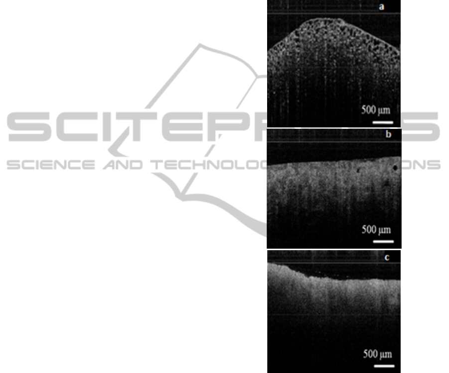
Figure 1: a) Normal Fat Tissue cross-section OCT image

(mature fat, adipose cells), logarithmic response. b) Well-

differentiated Fat Tissue cross-section OCT image (WDLS

with extensive myxoid change), logarithmic response. c)

De-differentiated Fat Tissue cross-section OCT image

(Highly fibrotic DDLS), logarithmic response.

The above images show the cross-section of

Human Normal Fat tissue (Figure 1a), WDLS

(Figure 1b) and DDLS (Figure 1c). This 2D cross-

section called B-scan is composed of 500 adjacent

A-lines. One A-line (1D) shows the backscattered

intensity variation in function of depth from a laser

footprint of 8 μm in focal plane. The region is 3mm

BIOIMAGING2014-InternationalConferenceonBioimaging

wide scanned with a galvanometer mirror, with

backscattered light collected from a region of up to

~1 mm in depth.

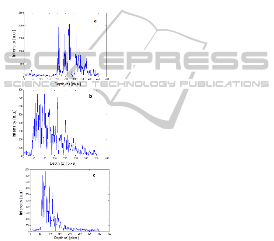
The internal structure is revealed. We can see the

differences of the different tissue types on the gray-

scale images. We intend to transform the qualitative

information from the images to a quantitative

statistical parametric description of the tissue. The

statistical model is based on the variability of the A-

lines in the cross-section at a given region. One A-

line of the different tissue types is seen on Figure 2.

Figure 2: OCT A-line of a) Normal Fat b) WDLS c)

DDLS. The intensity of the input laser light and the path-

length difference between the reference mirror and the

tissue surface differ in each case.

1D imaging (Intensity as a function of depth at a

single point) is obtained by applying Digital Signal

Processing methods on the data detected on a line

scan camera (Basler Sprint L104K-2k, 2048 pixel

resolution, 29.2 kHz line rate), -with a resolution of

2k, and a 10x10 μm2 pixel size, detecting 2048

wavelength intensity values between 800-890 nm.

The signal is digitized using an analog-to-digital

converter (NI-IMAQ PCI-1428). The intensity

detected on the line-scan camera is the cross-

correlation of the broadband laser light electric field

split in a Michelson interferometer and scattered

back from a reference mirror and from the sample

layers at each frequency component (Carbajal, 2011,

Drexler, 2008, Brezinski, 2006). The broadband

laser light is decomposed into its spectral

components in passing through a diffraction grating

(Wasatch Photonics, 1200 grooves/mm). The

measurement setting and DSP is computed in

Labview, whence the intensity functions as function

of depth are analyzed in Matlab.

3 DATA ANALYSIS

The post-processing steps to determine the model on

the Fourier-domain signatures derived from OCT

data will be explained here. Human Normal Fat,

WDLS and DDLS tissue samples will be analyzed.

We will focus on the statistical properties of the

backscattered intensity signals.

For the computation, the tissue surface should

first be numerically straightened. We apply the

canny edge detector implemented in Matlab Image

Processing Toolbox on the B-scans after median

filtering the images. This can be used to align the

scans, but does not yield the absolute position of the

surface with respect to common origin. Before

further analysis we screen all the B-scans to verify

that each one is straightened properly.

At each depth position the mean and standard

deviation of the intensity signals will be calculated.

Then, attenuation effects are removed from the data

by dividing the Intensity Values or the standard

deviation of the A-lines by the mean from each

backscattered intensity response, so as to normalize

every scan line.

The images are corrected according to the

normalized camera sensitivity curve, to eliminate the

errors coming from the intensity variations because

of the oblique tissue surface. It is due to the camera

feature recording the same sample point at lower

intensity from farther path-length differences

following a Gaussian decay (Bajraszewski, 2008).

3.1 Standard Deviation over Mean

In the first case the tissue characterization will be

defined from the Probability Density Functions

Model-basedApproachtoTissueCharacterizationusingOpticalCoherenceTomography

(PDF) of the STD/MEAN curves. The three-

parameter Generalized Extreme Value (GEV)

Distribution fits the histograms well due to its high

flexibility:





x|k,μ,σ













exp







1k



















1k















(2)

where x is the std/mean of the intemsity values, y is

the distribution, k is the shape-, σ is the scale-, μ is

the location parameter.

To find the tissue surface on the straightened

images the mean of the A-lines in one B-scan, and

the first derivatives of the mean are calculated from

the uncorrected images. The tissue surface is defined

at the highest derivative point.

After the tissue surface is defined, 150 pixel =

0.659 mm is considered for analysis because the

most dense tissue (DDLS) does not reflect light from

deeper region at this wavelength range and camera

settings (Figures 3a).

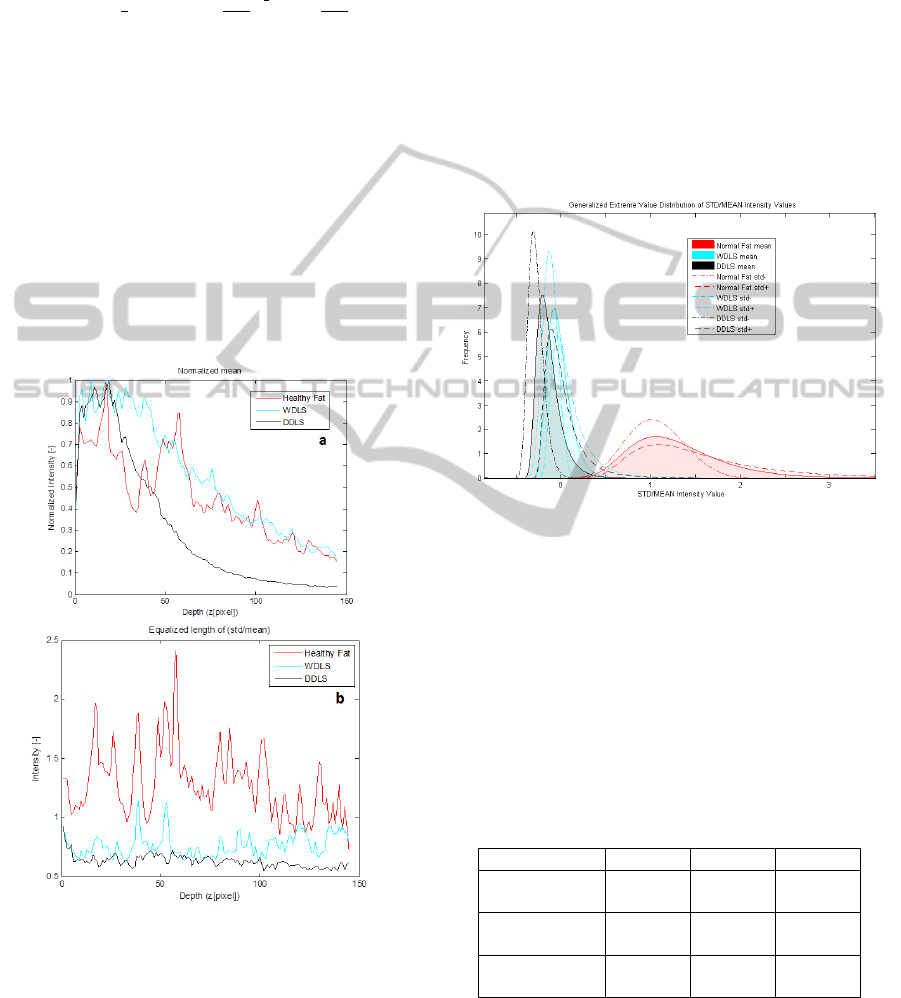
Figure 3: a) Averaged B-scan, mean intensity value at

each depth position on Normal Fat, WDLS, DDLS; (150

pixels from the tissue surface) The curves here are

normalized according to maximum value only for

representation. b) Standard Deviation over Mean at each

depth position in the same region.

The next step will be to define the Region of Interest

(ROI) on the curves for analysis. This analysis relies

on the use of a windowing scheme, in which

sections of the intensities as function of depth are

evaluated separately.

After evaluation of the data in each window

region at each B-scan via the parameters of the GEV

distribution, a window size of 40 pixel = 0.1758 mm

is chosen, beginning from the tissue surface. Our

method turned out to be independent on the surface

scattering effect.

To depict the accuracy of the results, 160 WDLS

or DDLS and 200 Normal Fat B-scans were

analyzed. Figure 4 shows the mean and STD of the

GEV parameters on the Gaussian corrected curves.

It characterizes well the different tissue types.

Figure 4: Histogram, GEV Distribution (k, σ, μ) calculated

from the STD/mean ratio of the intensity values at each

depth position in ROI, mean and standard deviation on

200 B-scans of Normal Fat, and 160 B-scans of WDLS

and DDLS.

The curve coefficients well differentiate between

the healthy and cancerous tissues, but there is less

distinction between the grades of the cancer (Table

1).

Table 1: GEV parameters calculated from the STD/MEAN

ratio of the intensity values at each depth position, mean

and standard deviation on 200 B-scans of Normal Fat, and

160 B-scans of WDLS and DDLS.

STD/MEAN k σ μ

Baseline

(Normal Fat)

0.0007

+0.2347

0.2151

+0.0579

1.2796

+0.0659

Deviation1

(WDLS)

-0.0128

+0.2443

0.0529

+0.0120

0.7093

+0.0359

Deviation2

(DDLS)

0.0857

+0.1673

0.0493

+0.0128

0.6502

+0.0584

To draw the deviation from the baseline tissue

the next parameters are calculated, where b is the

Baseline tissue parameter, d is the Deviated tissue

parameter.

BIOIMAGING2014-InternationalConferenceonBioimaging

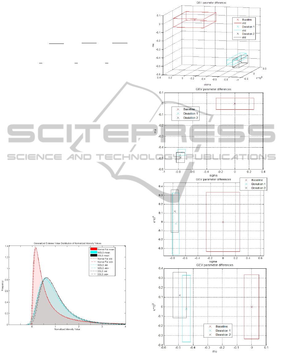
Table 2: Comparison of the GEV parameters calculated

from the STD/mean ratio of the intensity values at each

depth position, mean and standard deviation on 200 B-

scans of Baseline Tissue and 160 B-scans of Deviation

1&2.

STD/MEAN

∆













∆













∆













Baseline

(Normal Fat)

+335.2857

+0.2692

+0.0515

Deviation 1

(WDLS)

-19.2857

[-368.2857;

329.7143]

-0.7541

[-0.8099;

-0.6983]

-0.4457

[-0.4737;

-0.4176]

Deviation 2

(DDLS)

121.4286

[-117.5714;

360.4286]

-0.7708

[-0.8303;

-0.7113]

-0.4919

[-0.5375;

-0.4462]

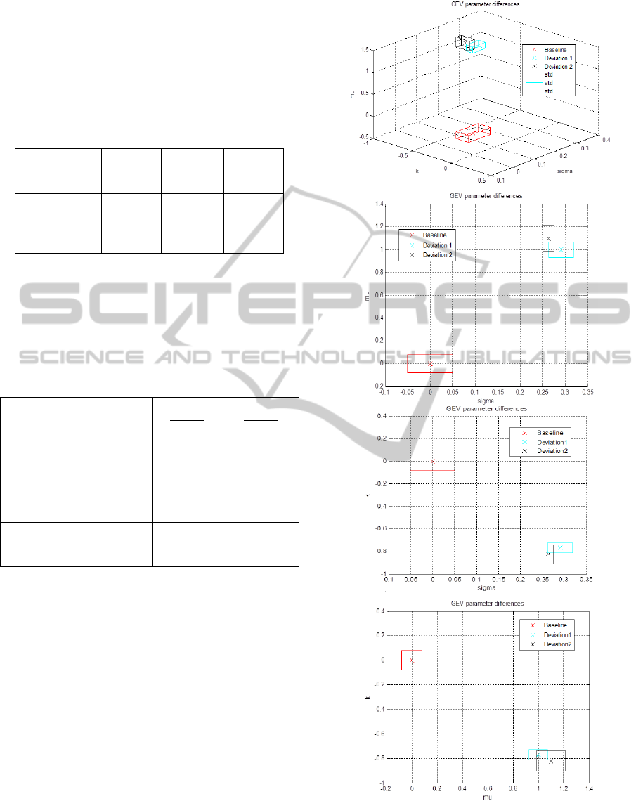
The next figure represents the coefficient

differences on the axes of a 3D coordinate system. It

is clear, that there is a relevant separation between

the healthy and cancerous tissue in each projection

plane.

3.2 Normalized Intensity Variation

A second method is developed to analyze the same

data set. Instead of calculating the STD/MEAN, all

the measured intensity values are now considered,

and also normalized by the mean intensity at each

depth position. The same windowing process was

applied on the A-lines and B-scans, and the optimal

window size of 40 pixels beginning from the surface

has been proved. Figure 6 and Table 3 shows the

mean and STD of the GEV parameters

characterizing the different tissue types.

Figure 6: Histogram, GEV Distribution (k, σ, μ) calculated

from the mean-normalized intensity values in ROI, mean

and standard deviation on 200 B-scans of Normal Fat, and

160 B-scans of WDLS and DDLS.

Figure 5: Comparison of the GEV parameters represented

at each axe of the 3D coordinate system calculated from

the STD/mean ratio of the intensity values at each depth

position, mean and standard deviation on 200 B-scans of

Baseline Tissue and 160 B-scans of Deviation 1&2.

Model-basedApproachtoTissueCharacterizationusingOpticalCoherenceTomography

Similarly to the first method the curve coefficients

characterize well the healthy and cancerous tissue

but WDLS and DDLS coefficients are not

sufficiently distinguished.

Table 3: GEV parameters calculated from the mean-

normalized intensity values in ROI, mean and standard

deviation on 200 B-scans of Normal Fat, and 160 B-scans

of WDLS and DDLS.

I/MEAN k σ μ

Baseline

(Normal Fat)

0.8209

+0.0647

0.3532

+0.0181

0.3191

+0.0254

Deviation1

(WDLS)

0.1905

+0.0358

0.4561

+0.0100

0.6381

+0.0229

Deviation2

(DDLS)

0.1447

+0.0684

0.4462

+0.0044

0.6700

+0.0364

The next table shows the deviation from the

baseline tissue, where b is the Baseline tissue

parameter, d is the Deviated tissue parameter.

Table 4: Comparison of the GEV parameters calculated

from the mean-normalized intensity values in ROI, mean

and standard deviation on 200 B-scans of Baseline Tissue

and 160 B-scans of Deviation 1&2.

ΣI /MEAN

∆















∆















∆















Baseline

(Normal

Fat)

+0.0788

+0.0512

+0.0796

Deviation1

(WDLS)

-0.7679

[-0.8115;

-0.7243]

0.2913

[0.2630;

0.3196]

0.9997

[0.9279;

1.0715]

Deviation2

(DDLS)

-0.8237

[-0.9071;

-0.7404]

0.2633

[0.2508;

0.2758]

1.0997

[0.9856;

1.2137]

The next figure shows similar results then the

first method representing the coefficient differences

in the 3D coordinate system and separating well the

healthy and cancerous tissue in each projection

plane, however the different cancer tissues are

overlapped.

4 DISCUSSION

We can deduce that both statistical analyses are a

viable method to differentiate tissue types with a

good accuracy. The method is independent on the

measurement settings as the results are normalized

by the mean of the intensity values at each depth

position, and errors due to path-length differences

are corrected. For comparison the data analysis was

also applied on the images without this correction

Figure 7: Comparison of the GEV parameters represented

at each axe of the 3D coordinate system calculated from

the mean-normalized intensity values in ROI, mean and

standard deviation on 200 B-scans of Baseline Tissue and

160 B-scans of Deviation 1&2.

BIOIMAGING2014-InternationalConferenceonBioimaging

revealing that only the shape parameter (k) is

affected in a non-negligible way in the case the

STD/MEAN ratio is calculated. This analysis is

more sensitive also to the way how we find the

surface of

the tissue since the data points from

which the histogram is drawn is deduced calculating

the STD/MEAN from each depth position (40

pixels), comparing to the second method where the

histogram is drawn from the data points contained in

all the Region of Interest (40x200 or 40x160 pixel

points). In case we want to get absolute parameters,

which describe tissue type, the correction is needed.

The method could be developed to distinguish

better the different grade of cancer implementing

with additional factors, e.g. the mean intensity

values at each depth position. The weak point of the

measurements is that setting the position of the

tissue under the laser light to get a visible subsurface

structure is controlled manually. The measurements

revealed that the focus position does not affect

significantly the quantitative results, but some

saturated intensity points can also affect the

statistics.

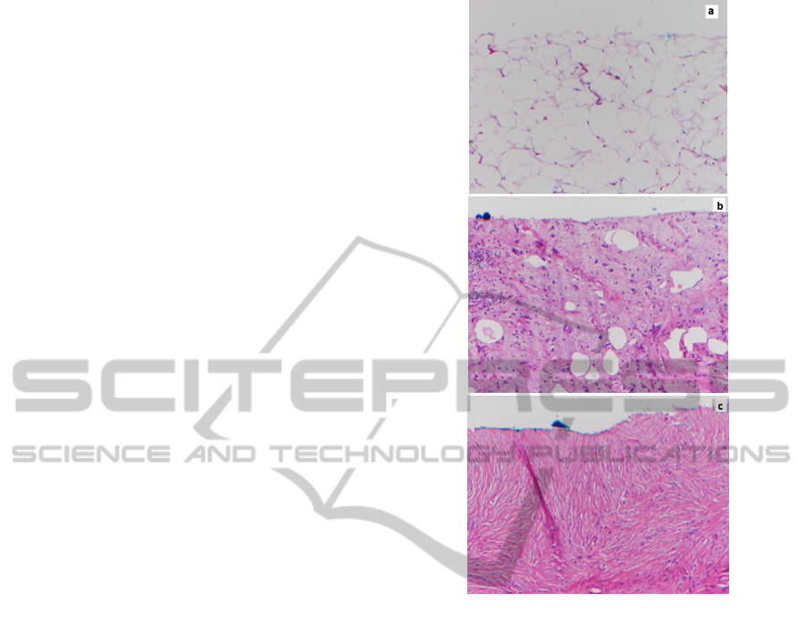
It has already been proved that this non-invasive

measurement technique shows good similarities with

stained histology (Figure 8) (Lev, 2011). The

novelty of our study was to develop a mathematical

model-based approach instead of visual grading of

the structure to be able to differentiate tissue types.

The structure is detected from the scattering

properties of the tissue types. The laser clearly

reveals the adipose cells seen in Normal Fat. WDLS

has extensive myxoid change including vasculature,

but still has some adipose cells with varying size,

which is a diagnostic of WDLS. The part of DDLS

imaged here resembles fibrotic tissue.

Cancerous tissue is much denser than healthy

tissue. Since light scattering occurs chiefly at

interfaces, scattering is much stronger in cancerous

tissue. The inhomogeneous Normal Fat is

distinguished with periodic scattering at the cell

boundaries. The attenuation of light is higher in the

dense tissue, detectable with the attenuation

coefficient 



, and the back reflection loses the

periodicity as the adipose cells dedifferentiate in the

cancerous tissue. The optical properties show the

morphology of the tissues, the scattering effects

reveal the cellular structure at a good resolution for

our analysis.

For medium grade sarcoma (WDLS), there is

much larger cell size dispersion than in healthy

tissue. An analysis of the structure’s periodicities is

sensitive to this, as well as speckle analysis. Cell

counting analysis can reveal the difference between

Figure 8: Histological images (Magnification 10x) of a)

Normal Fat b) Well-Differentiated Liposarcoma with

extensive mitotic change c) Highly Fibrotic De-

Differentiated Liposarcoma.

healthy tissue and high grade of cancer (DDLS), the

size of the variable adipose cells should be included

in the algorithm to distinguish between normal fat

and medium grade of cancer (WDLS). It can be

improved using artificial network analysis already

calculated on histological data (Sjöström, 1999).

There is a certain degree of order (on a given length

scale) in healthy tissue. On the contrary, in sarcoma,

many scales are present, which is revealed by fractal

analysis.

The techniques proposed in literature have not

been applied in clinical practice yet and there are

some shortcomings in the analysis. The slope

analysis discards all structural information; the

fractal analysis is too complicated and subject to

erroneous or ambiguous interpretation due to

experimental errors. The speckle analysis discards

information on loss of intensity due to multiple

scattering events. Finally it seems likely that

completely automated, practicable cell counting

Model-basedApproachtoTissueCharacterizationusingOpticalCoherenceTomography

analysis will not be achieved using traditional image

analysis software.

The aim of our study is to develop a simple

analysis technique based on a parametric method

that captures the structural features from the strength

of scattering. Here only one histological subtype of

WDLS and DDLS is described, however they can

represent several patterns (Miettinen, 2003,

Miettinen, 2010) The comparison of the different

histological subtypes and the ability to differentiate

from Normal Fat and Lipoma, benign adipose tissue

is a future study.

5 CONCLUSIONS

Our objective was to study the response of tissue to

a near infrared laser excitation, and, specifically, to

characterize differences between healthy and

cancerous tissue. The morphology of the subsurface

is depicted based on the backscattered near infrared

light. Parametric models of these backscattered

signal characteristics are derived and linked

statistically to the optical properties of Normal Fat,

Well-Differentiated Liposarcoma and De-

Differentiated Liposarcoma.

The accurate diagnosis at early stage of cancer,

as well as the recognition of the tumor boundary in

tissue is highly important. However OCT has been

well-recognized as a powerful method for cancer

detection from tissue morphology, the diagnosis

from these images is subjective and not obvious. We

intend to fill the need for an objective means of data

analysis. The goal of the current study was to

develop a quantitative diagnostic method

differentiating between healthy and cancerous tissue.

The data analysis is developed on images

recorded on human Normal Fat Tissue vs. Well-

differentiated (WD) and De-differentiated

Liposarcoma (DDLS). Further refinement will allow

to detect tumor boundary, diagnose other type of

cancer (e.g. breast cancer) where structural analysis

is required for diagnosis, or to monitor quantitatively

tumor progression during cancer therapy.

As a demonstration of these methods, statistical

analysis was developed to evaluate OCT images of

human fat specimens. An accurate result was found

to quantify healthy vs. cancerous tissue. The analysis

can be applied in real-time for diagnosis, and it is

much simpler comparing to other quantifying

method. This practical advantage gives a good

possibility to use in surgical evaluation.

We describe first time a model-based tissue-

characterization method based on structural

properties of healthy vs. cancerous tissue. Further

statistical validation, sensitivity/specificity analysis

and classification methods have to be performed on

other measurements to prove the efficacy of the

developed method.

ACKNOWLEDGEMENTS

The authors wish to acknowledge the very important

contribution made by Shang Wang and Narendran

Sudheendran. This work was supported by the

Hungarian-American Fulbright Commission, the

French Ministry of Research and the University of

Houston. This work is the continuation of a poster

presentation held on November 16, 2012 at the

MEGA Research day of the University of Houston.

REFERENCES

Bajraszewski, T., Wojtkowski, M., Szkulmowski, M.,

Anna Szkulmowska, Huber, R., Kowalczyk, A., 2008.

Improved spectral optical coherence tomography using

optical frequency comb, Optics Express, 16(6).

Brezinski, M. E., 2006. Optical Coherence Tomography,

Principles and Applications, Academic Press Elsevier

Inc.

Drexler, W. and Fujimoto, J. G., 2008. Optical Coherence

Tomography: Technology and Applications, Springer,

Berlin, New York.

Carbajal, E. F., Baranov, S. A., Manne, V. G. R., Young,

E. D., Lazar, A. J., Lev, D. C., Pollock, R. E., Larin,

K.V., 2011. Revealing retroperitoneal liposarcoma

morphology using optical coherence tomography,

Journal of Biomedical Optics, 16(2).

Fletcher, C. D. M., Rydholm, A., Singer, S., Sundaram,

M., Coindre, J. M., 2006. Soft tissue tumours:

Epidemiology, clinical features, histopathological

typing and grading, WHO Classification of Soft Tissue

Tumors.

Goldberg, B. D., Iftimia, N. V., Bressner, J. E., Pitman, M.

B., Halpern, E., Bouma, B. E., Tearney, G. J., 2008.

Automated algorithm for differentiation of human

breast tissue using low coherence interferometry for

fine needle aspiration biopsy guidance, Journal of

Biomedical Optics, 13(1),

Gossage, K. W., Tkaczyk, T. T., Rodriguez, J. J., Barton,

J. K., 2003. Texture analysis of Optical Coherence

Tomography images: feasibility for tissue

classification, Journal of Biomedical Optics, 8(3).

Gossage, K. W., Smith, C. M., Kanter, E. M., Hariri, L. P.,

Stone, A. L., Rodriguez, J. J., Williams, S. K., Barton,

J. K., 2006. Texture analysis of speckle in Optical

Coherence Tomography images of tissue phantoms,

Physics in Medicine and Biology. 51.

BIOIMAGING2014-InternationalConferenceonBioimaging

Lahat, G., Madewell, J.E., Anaya, D. A., Qiao, W., Tuvin,

D., Benjamin, R. S., Lev, D. C., and Pollock, R. E.,

2009. Computed Tomography Scan-Driven Selection

of Treatment for Retroperitoneal Liposarcoma

Histologic Subtypes, Cancer 115(5).

Lev, D., Baranov, S. A., Carbajal, E. F. Young, E. D.,

Pollock, R. E., Larin, K. V., 2011. Differentiating

retroperitoneal liposarcoma tumors with optical

coherence tomography, Proceedings SPIE 7890,

Advanced Biomedical and Clinical Diagnostic

Systems IX, 78900U.

McLaughlin, R. A., Scolaro, L., 2010. Parametric imaging

of cancer with optical coherence tomography, Journal

of Biomedical Optics, 15(4).

Miettinen, M. M., 2003. Diagnostic Soft Tissue Pathology,

Churchill Livingstone.

Miettinen, M. M., 2010. Modern soft tissue pathology;

tumors and non-neoplastic conditions, Cambridge

University Press.

Morris, P., Perkins, A., 2012. Diagnostic imaging, Physics

and Medicine 2, Lancet, 379.

Mujat, M., R., Ferguson, D., Hammer, D. X., Gittins, C.,

Iftimia, N., 2009. Automated algorithm for breast

tissue differentiation in optical coherence tomography,

Journal of Biomedical Optics, 14(3).

Rembielak, A., Green, M., Saleem, A., 2011. Pat Price,

Diagnostic and therapeutic imaging in oncology,

Cancer Biology and Imaging, Medicine, 39(12).

Sjöström, P. J., Frydel, Wahlberg, L. U., 1999. Artificial

Neural Network-Aided Image Analysis System for

Cell Counting, Cytometry, 36.

Sullivan, A. C., Hunt, J. P., Oldenburg, A. L., 2011.

Fractal analysis for classification of breast carcinoma

in Optical Coherence Tomography, Journal of

Biomedical Optics, 16(6).

Yang, Y., Wang, T., Biswal, N.C., Wang, X., Sanders, M.,

Brewer, M., Zhu, Q., 2011. Optical scattering

coefficient estimated by optical coherence tomography

correlates with collagen content in ovarian tissue,

Journal of Biomedical Optics, 16(9).

Zysk, A. M., Boppart, S. A., 2006. Computational

methods for analysis of human breast tumor tissue in

optical coherence tomography images, Journal of

Biomedical Optics, 11(5).

Model-basedApproachtoTissueCharacterizationusingOpticalCoherenceTomography