
Comparison of Performances of Plug-in Spatial Classification Rules
based on Bayesian and ML Estimators
Kestutis Ducinskas, Egle Zikariene and Lina Dreiziene
Department of Matematics and Statistics, Klaipeda University, Herkaus Manto str. 84, Klaipeda, Lithuania
Keywords: Bayes Rule, Spatial Discriminant Function, Gaussian Random Field, Actual Risk, Training Labels
Configuration.
Abstract: The problem of classifying a scalar Gaussian random field observation into one of two populations specified
by a different parametric drifts and common covariance model is considered. The unknown drift and scale
parameters are estimated using given a spatial training sample. This paper concerns classification
procedures associated to a parametric plug-in Bayes Rule obtained by substituting the unknown parameters
in the Bayes rule by their estimators. The Bayesian estimators are used for the particular prior distributions
of the unknown parameters. A closed-form expression is derived for the actual risk associated to the
aforementioned classification rule. An estimator of the expected risk based on the derived actual risk is used
as a performance measure for the classifier incurred by the plug-in Bayes rule. A stationary Gaussian
random field with an exponential covariance function sampled on a regular 2-dimensional lattice is used for
the simulation experiment. A critical performance comparison between the plug-in Bayes Rule defined
above and a one based on ML estimators is performed.
1 INTRODUCTION
It is known that for completely specified populations
and loss function, Bayes Rule (BR) is an optimal
classification procedure in the sense of minimum
risk (expected losses) (Anderson, 2003). When this
is not the case, the missing information is usually
provided by a training sample. For parametrically
specified populations, the training sample is used to
obtain the estimators of statistical parameters and
plugging them into the BR. The resulting
classification rule is usually called a plug-in Bayes
rule (PBR). Actual risk (ACR) or conditional risk is
usually used as a performance measure for the PBR.
Performance comparison of the PBR based on the
different types of estimators can easily be done by
the closed-form expression of the ACR.
Many authors have investigated the performance
of the PBR when the parameters are estimated from
training samples consisting of dependent
observations by using the frequentist approach for
the estimation (Kharin, 1996; Saltyte-Benth and
Ducinskas, 2005; Batsidis and Zografos, 2011). A
closed-form expression for the ACR in supervised
classification of Gaussian random field observations
is derived by Ducinskas (2009). Only the ML
estimators of the drift parameters and the scale
parameter of covariance function are considered.
In the present paper we use Bayesian estimators
instead of the ML estimators for the classification
problem described above. Proposed methodology is
useful for classification of images corrupted by the
Gaussian spatial correlated noise (Ducinskas,
Stabingiene and Stabingis, 2011).
The closed-form expression for the ACR
associated with the PBR is derived. The estimator of
expected risk is based on the derived actual risk and
is used as the performance of the PBR which is
measured by the average of the ACR usually called
an empirical estimator of expected risk.
This estimator of expected risk is a case of the
stationary Gaussian random field on 2-dimentional
regular lattice with an exponential covariance
function. The dependence of the ACR values on the
statistical hyperparameters is investigated.
Numerical comparison for the case of ML estimators
is implemented.
161
Ducinskas K., Zikariene E. and Dreiziene L..
Comparison of Performances of Plug-in Spatial Classification Rules based on Bayesian and ML Estimators.
DOI: 10.5220/0004760701610166
In Proceedings of the 3rd International Conference on Pattern Recognition Applications and Methods (ICPRAM-2014), pages 161-166
ISBN: 978-989-758-018-5
Copyright
c
2014 SCITEPRESS (Science and Technology Publications, Lda.)

2 THE MAIN CONCEPTS AND
DEFINITIONS
This paper concerns classifying a Gaussian random
field (GRF)
:
p
s
sD RZ observations into one
of two populations denoted by
12
,.
The model of an observation
Z
s
in a
population
j
is
j
Z
sss
(1)
where
j
s
, is a drift (a deterministic function of
locations) and
s
is the stochastic error term,
j=1,2.
Suppose the drift
j
s
can be represented as
j
j
s
x
,where x is a 1q vector of non-
random regressors and
j
β
is a 1q vector of the
parameters,
1, 2j .
The error term is generated by a zero mean
stationary GRF
:
s
sD
with the covariance
function defined by the model for all
,
s
uD
2
cov ,
s
uCsu
,
(2)
where
2
is the variance or the scale parameter and
C is the spatial correlation function.
In the case when the covariance function
parameters are known, the model (1), (2) is called a
universal kriging model (Cressie, 1993).
For the given training sample, consider the
classification problem of the
00
()
Z
Zs into one of
two populations when
01 020
,.
x
sxssD
Denote by
;1,...,
ni
SsDi n
the set of
locations where the training sample
1
'((),...,())
n
TZs Zs is taken. It specifies the spatial
sampling design or the spatial framework for the
training sample (Shekhar et al., 2002).
We shall assume the deterministic spatial
sampling design and all analyses are carried out
conditional on
n
S .
Assume that each training sample realization
T=t
and
n
S are arranged in the following way. The first
1
n components are the observations of
Z
s
from
1
and the remaining
21
nnn components are
the observations of
Z
s
from
2
. So
n
S is
partitioned into a union of two disjoint subsets, i. e.
(1) (2)
n
SS S, where
()
j
S is a subset of
n
S that
contains
j
n
locations of the feature observations
from
j
,
1, 2j
. So each partition
(1) ( 2)
() ,
n
SSS
with marked labels determines
the training labels configuration (TLC).
For TLC
()
n
S
, define the variable
(1) (2)
dD D, where
()j
D is a sum of distances
between the location
0
s
and the locations in
()
j
S
,
1, 2j
.
The
2nq
design matrix of the training sample
T denoted by X is specified by
12
X
XX, where
the symbol
denotes a direct sum of the matrices
and
j
X
is a
j
nq
matrix of the regressors for the
observations from
j
, 1, 2j
.
As it follows, we assume that
n
S and TLC
n
S
are fixed. This is the case, when spatial
classified training data are collected at the fixed
locations (stations).
So the model of the training sample is
TX E
,
(3)
where
12
,
is a 21q vector of the
regression parameters and
E is the
n
- vector of the
random errors that has a multivariate Gaussian
distribution
2
0,
nn
NC
.
Here
n
C denotes a spatial correlation matrix
among the observations forming the training sample
T .
Denote by
0
c the vector of correlations among
0
Z
and the components of T. Let t denote the
realization of
T .
Since
0
Z
follows the model specified in (1), the
conditional distribution of
0
Z
given ,
j
Tt,
1, 2j
is Gaussian with the mean
0
000
;
lt j j
EZ T t x t X
(4)
and the variance
22
00
var ;
tj
ZT t
,
(5)
where
00
()
x
xs
,
1
00
n
cC
,
1
000
(1 )
n
cC c
.
Under the assumption of complete parametric
certainty of populations and for known finite non-
negative losses
,,, 1,2Lij ij , BR minimizing
the risk of classification is associated with the spatial
ICPRAM2014-InternationalConferenceonPatternRecognitionApplicationsandMethods
162

discriminant function (SDF) formed by a log ratio of
conditional likelihoods (McLachlan, 2004).
00
0012
00 2
12
1
,
2
,
ttt
ttt
WZ Z
(6)
where
**
12
ln
and
2
,
.
Here
*
,3 ,
jj
Lj j Ljj
, 1, 2j
,
where
12 1 2
,1
are prior probabilities of
the populations
1
and
2
, respectively.
Note, that in the present paper we implemented
the following values of the prior probabilities
ˆ
/, 1,2.
jj
nnj
So the classification procedure based on the SDF
allocates the observation in the following way:
Classify the observation
0
Z
given Tt to the
population
1
if
0
,0
t
WZ
, and to the
population
2
, otherwise.
Definition 1. The risk for the classification rule
based on the SDF
0
;
t
WZ
is defined as
22
0
11
,
iij
ij
RLijP
,
(7)
where, for
,1,2ij ,
0
1;0
j
ij it t
PP WZ
.
Here, for
1, 2i
, the probability measure
it
P is
based on the conditional distribution of
0
Z
given
Tt ,
i
specified in (4), (5).
Note that under the condition (3), the squared
Mahalanobis distance between
1
and
2
in the
location
0
s
based on marginal distributions of
0
Z
and the same squared Mahalanobis distance given
Tt are specified by
2
200 2
12
/)
and
2
200 2
012
/
tt t
, respectively.
From (4), (5) it follows that
22
00
/
. In the
population
j
, the conditional distribution of
0
;
t
WZ
given Tt is the normal distribution
with the mean
12
00
;(1)/2
j
jt
EWZ
and the variance
2
00
;,1,2.
jt
Var W Z j
By using the properties of normal distributions
we obtain
2
*
000
1
21 (,),
j
jj
j
RLjj
where
is the standard normal distribution
function.
In practical applications not all statistical
parameters of populations are known. In such cases
the estimators of the unknown parameters can be
found from the training sample. When the estimators
of the unknown parameters are plugged into the
SDF, the plug-in SDF (PSDF) is obtained. In this
paper we assume that the true values of the
parameters
and
2
are unknown (complete
parametric uncertainty).
Let
2
ˆ
ˆ
,
be the estimators of the
corresponding parameters from the training sample.
Put
2
ˆ
ˆ
ˆ
,.
After replacing the parameters
with their estimates in (6) the PSDF gets the
following form
000 0
2
00
1
ˆˆ
ˆ
;
2
ˆ
ˆ
()
t
WZ Z t X xH
xG
(8)
with
,
qq
H
II and
,
qq
GII, where
q
I
denotes the identity matrix of the order q.
Definition 2. The expectation of the ACR with
respect to the distribution of T is called the expected
risk (ER).
Recall that the actual risk incurred by the PSDF
is obtained by replacing
by the ML estimator
ˆ
in (6) (Ducinskas and Dreiziene, 2011).
Lemma 1. The actual risk for
0
ˆ
;
t
WZ
specified in (8) is
2
*
1
ˆ
ˆ
,
Ajjj
j
RQLjj
,
(9)
where
2
00000
ˆ
ˆˆˆ
ˆ
1( )sgn( )/ /
j
jj
QabxG xG
and
00
()
jj
ax tX
,
00
ˆ
ˆˆ
(2)btXxH
for 1, 2j .
The proof of the lemma is presented in the
appendix.
The ACR is useful in providing a guide to the
performance of the plug-in classification rule when
it actually formed from the training sample. The ER
is the performance measure to the PBDF similar as
the mean squared prediction error (MSPE) is the
performance measure to the plug-in kriging
predictor (Diggle, Ribeiro and Christensen, 2002).
The estimators of the MSPE are used for the spatial
sampling design criterion for the prediction
ComparisonofPerformancesofPlug-inSpatialClassificationRulesbasedonBayesianandMLEstimators
163

(Zimmerman, 2006; Zhu and Zhang, 2006). These
facts strengthen the motivation for the deriving of
the estimators of the ER associated with the PSDF.
In this paper we propose an empirical estimator
of the ER incurred by the rule based on the proposed
PSDF. The following steps are performed to
construct this estimator:
1.
Simulate M training sample T realizations
according to the model specified in (3).
2.
For each simulated realization of
l
Tt
,
1,lM compute the appropriate estimates
ˆ
l
and
2
ˆ
l
, respectively. Set
2
ˆ
ˆ
ˆ
,
lll
3.
By using (9) compute the empirical estimator of
the ER
1
()
ˆ
ˆ
M
l
l
A
RR M
,
(10)
where
- denotes the abbreviation of the estimator
type, i.e. takes the values BA or ML.
3 THE ESTIMATORS OF
PARAMETERS
It is known, that the ML estimators of
and
2
based on T are
1
11
ˆ
ML
XR X XR T
,
21
ˆˆ
ˆ
ML ML ML
TX RTX n
.
Using the properties of the multivariate Gaussian
distribution is easy to prove that
2
ˆ
~,
ML q
N
,
1
21
XR X
222
2
ˆ
~2
ML n q
nq
.
The ML estimator of
and the bias adjusted
ML estimator of
2
are used in the PLDF, i.e.
ˆˆ
M
L
,
22
ˆˆ
2
ML
nn q
(Ducinskas, 2009).
In the Bayesian approach the likelihood is given
by
22
,~ ,
n
TNR
. The conjugate prior are
chosen for the parameters so
222
,ppp
, where
00
22
2
~,
q
pN
is the Gaussian prior
for
conditional on
2
,
00
2
~,pIGuv
–
the prior density for
2
, where
00
,0uv .
So the conjugate prior is the Normal–Inverse
Gamma (NIG) and denotes as
0000
,,,NIG u v
. Combining the prior with
the likelihood gives a joint Normal–Inverse Gamma
posterior (Diggle, Ribeiro and Christensen, 2002):
22
1111
2
,,
,,,,
ppT
p
TNIGuv
pT
where
1
11
10 00
11TT
XRX XRT
,
1
1
10
1T
XRX
,
10
2
n
uu
,
11
10 0 0 0 1 1 1
1
1
.
2
vv TRT
The marginal posterior for
on integrating out
2
is a multivariate Student distribution
1
~,
p
pTt
, where
1
2pu
,
11 1
vu
.
The marginal posterior for
2
is
11
2
~,pTIGuv
, where
,IG .
So the BA of
and
2
are
1
ˆ
BA
,
11
2
ˆ
1
BA
vu
, respectively.
4 EXAMPLE AND DISCUSSIONS
A numerical example is considered to investigate the
influence of the parameter estimation methods to the
proposed empirical estimator of the ER in the finite
(even small) training sample case. With an
insignificant loss of generality a case with
,1,,1,2
ij
Lij ij
is considered.
In this example, the observations are assumed to
arise from the stationary Gaussian random field with
the constant mean and the exponential correlation
function specified by
expch h
is
considered. Here
denotes the range parameter.
Assume that D is a regular 2-dimentional lattice with
unit spacing. Consider the case of
0
(1, 1)s and the
fixed set of training locations
8
S containing 8
second-order neighbours of
0
s
. This example also
illustrates the comparison of two different TLC.
Consider two TLC
1
,
2
for
8
S specified by
(1) (2)
1
(0, 2), (1,2),(2, 2), (2,1) , (2, 0), (1, 0), (0, 0),(0,1) .SS
ICPRAM2014-InternationalConferenceonPatternRecognitionApplicationsandMethods
164

(1) (2 )
2
(0, 2),(1, 2), (2, 2),(2,1), (2,0) , (1, 0),(0, 0),(0,1) .SS
These are illustrated in Figure 1.
Figure 1: Two different TLC with
1
S and
2
S points
marked as dots and asterisks.
By the definition, variable d represents the
asymmetry of the TLC with respect to the location
0
s
. It is easy to obtain that
0d
and
1
4n for
1
and
22d
with
1
5n for
2
.
So we can conclude that
1
is the symmetric TLC
and
2
is the asymmetric one. Denote by
()
ˆ
M
L
R and
()
ˆ
B
A
R
the empirical estimators of the ER given in
(10) with the implemented ML and BA parameter
estimators, respectively.
The values of the empirical estimators of
()
ˆ
R
are presented for
1
with
1
0, 5
, and for
2
with
1
5
8
in Table 1. Two cases of the simulated
realizations of the training sample are selected here,
i.e.
2
10M and
4
10M . Analyzing the figures of
the number of simulated realizations of the training
sample in Table 1 we see that for all
0.5, 0.7, ..., 1.9 values
() ()
ˆ
ˆ
M
LBA
RR . So we
can conclude that the BA case has an advantage
against the ML case by the ER minimum criterion.
The quantitative comparison of the two cases of the
parameter estimators is also done by the values of
the index
() ()
ˆˆ
M
LBA
RR
. The values of this index
are shown in Figure 2 for
4
10M and ,1,2.
l
l
It is easy to see from Figure 2 that for both the
TLC
1
and the values of this index increases
when
increases. The same situation is for both
TLC considered
.
5 CONCLUSIONS
In this paper, the comparison of two approaches to
parameter estimation is done based on the values of
the ER incurred by the classification rule based on
the PSDF.
The proposed optimality criterion is based on the
derived formula of the actual risk.
The simulation experiment shows the advantage
of Bayesian estimation approach against the
frequentist (ML) approach. This advantage is greater
for strongly separated populations (larger values of
) than for the close populations. These
conclusions are valid to the symmetric training
labels configuration as well to the asymmetric one.
Hence the results of this paper give us strong
arguments to expect that Bayesian estimators of
spatial population parameters could be effectively
used in spatial Gaussian data classification incurred
by plug-in Bayes rules.
Table 1: Values of
()
1
R
for the different estimators and the TLC
1
and.
2
.
1
1
ML BA ML BA ML BA ML BA
\
M
2
10
4
10
2
10
4
10
0.5 0.352 0.335 0.365 0.349 0.359 0.340 0.328 0.315
0.7 0.275 0.262 0.277 0.256 0.310 0.280 0.257 0.239
0.9 0.195 0.177 0.201 0.180 0.196 0.182 0.189 0.171
1.1 0.143 0.123 0.140 0.122 0.143 0.119 0.136 0.118
1.3 0.094 0.083 0.098 0.083 0.097 0.085 0.097 0.081
1.5 0.067 0.053 0.067 0.055 0.061 0.051 0.066 0.053
1.7 0.049 0.035 0.047 0.036 0.044 0.034 0.047 0.035
1.9 0.034 0.024 0.033 0.024 0.033 0.024 0.032 0.023
ComparisonofPerformancesofPlug-inSpatialClassificationRulesbasedonBayesianandMLEstimators
165
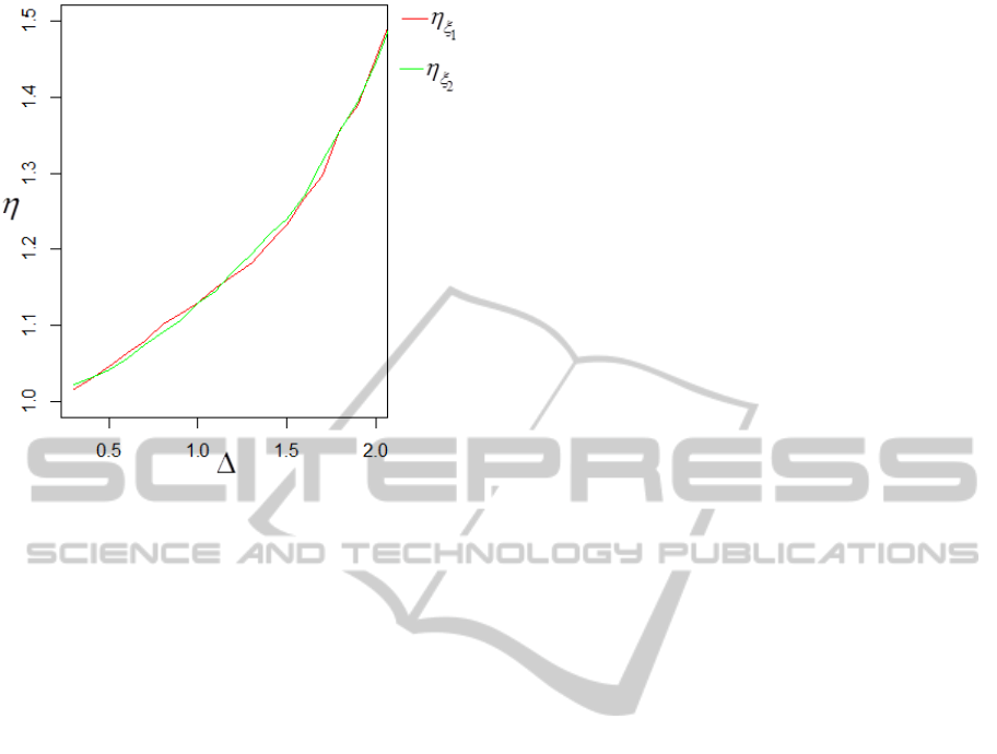
Figure 2: Values of
for different TLC.
REFERENCES
Anderson, T. W., 2003. An Introduction to Multivariate
Statistical Analysis
, Wiley. New York.
Batsidis, A. and Zografos, K., 2011. Errors of
misclassification in discrimination of dimensional
coherent elliptic random field observations.
Statistica
Neerlandica
, 65, p. 446-461.
Cressie, N. A. C., 1993.
Statistics for spatial data, Wiley.
New York.
Diggle, P. J., Ribeiro, P. J. and Christensen, O. F., 2002.
An introduction to model-based geostatistics.
Lecture
notes in statistics
, 173, p. 43-86.
Ducinskas, K., 2009. Approximation of the expected error
rate in classification of the Gaussian random field
observations.
Statistics and Probability Letters, 79,
p. 138-144.
Ducinskas, K., Dreiziene, L., 2011. Supervised
classification of the scalar Gaussian random field
observations under a deterministic spatial sampling
design.
Austrian Journal of Statistics. 40, No. 1, 2,
p. 25-36.
Ducinskas, K. Stabingiene, L., Stabingis, G., 2011. Image
classification based on Bayes discriminant functions.
Procedia Environmental Sciences, 7, p. 218-223.
Kharin, Y., 1996.
Robustness in Statistical Pattern
Recognition
, Kluwer Academic Publishers. Dordrecht.
McLachlan, G. J., 2004.
Discriminant analysis and
statistical pattern recognition
, Wiley. New York.
Saltyte-Benth, J. and Ducinskas, K., 2005. Linear
discriminant analysis of multivariate spatial-temporal
regressions.
Scandinavian Journal of Statistics, 32,
p. 281 – 294.
Shekhar, S., Schrater, P. R., Vatsavai, R. R., Wu, W. and
Chawla, S., 2002. Spatial Contextual Classification
and Prediction Models for Mining Geospatial Data.
IEEE Transactions on Multimedia, 4, p. 174-188.
Zhu, Z. and Zhang, H., 2006. Spatial sampling design
under infill asymptotic framework.
Environmetrics,
17, p. 323-337.
Zimmerman, D. L., 2006. Optimal network design for
spatial prediction, covariance parameter estimation,
and empirical prediction.
Environmetrics, 17, p. 635-
652.
APPENDIX
Proof of Lemma. Recall that the actual risk (ACR)
for PSDF
0
ˆ
;
t
WZ
(Ducinskas and
Dreiziene, 2011) is defined as
22
11
ˆˆ
,
iij
ij
RLijP
where for ,1,2ij
,
0
ˆ
1;0
j
ij it t
PP WZ
.
In the population
j
, it is easy to derive that the
conditional distribution of
0
ˆ
;
t
WZ given Tt
is
normal distribution with the mean
2
000
ˆ
ˆ
ˆ
ˆ
;/
jt j
EWZ a bxG
(14) and
the variance
2
24
0000
ˆ
ˆ
ˆ
;/
jt
Var W Z x G
,
1, 2j
.
Then by using the properties of the normal
distribution and we complete the proof of lemma 1.
ICPRAM2014-InternationalConferenceonPatternRecognitionApplicationsandMethods
166
