Optimal Fixed Interval Satellite Range Scheduling
Antonio J. Vazquez
1
and R. Scott Erwin
2
1
National Research Council Post-Doctoral Fellow, Albuquerque, NM, U.S.A.
2
Principal Research Aerospace Engineer, Air Force Research Laboratory, Albuquerque, NM, U.S.A.
Keywords:
Scheduling Algorithm, Polynomial Time Algorithm, Earth Observation Satellite, Ground Station Network.
Abstract:
The satellite scheduling community has provided several algorithms for allocating interaction windows be-
tween ground stations and satellites, from simple greedy approaches to more complex hybrid-genetic or
Lagrangian-relaxation techniques. Single-location ground station problems, where requests have fixed time
intervals and no priorities, are known to be solvable in polynomial time. To the best of our knowledge, no
algorithm has been provided yet for solving multiple-location, prioritized scheduling problems optimally. We
present an exact polynomial time algorithm for a fixed number of ground stations (or satellites), based on a
modified algorithm from the general scheduling literature.
1 INTRODUCTION
The problem of scheduling interactions between
ground stations and satellites is widely-known in
the literature as Satellite Range Scheduling (SRS).
Whereas ground stations can be considered to be
moving with the surface of the Earth, satellites travel
through different kinds of orbits. These two differ-
ent motion dynamics generate visibility time win-
dows when lines ofsight (LOS) between satellites and
ground stations exist.
The interactions are limited to occur within these
visibility windows, and could also involve time con-
straints specified by the operators of the satellites,
which depending on the specific mission may require
fixed or variable contact times lasting for the entire
window duration or just a portion of it.
In this paper we focus on the case where these
windows are defined by fixed times, so for the sake
of simplicity we assume that the passes are gener-
ated directly from the LOS times among ground sta-
tions and satellites. That is generally the case for Low
Earth Orbits (LEOs), due to their short times (L. Bar-
bulescu, 2004) (for more insight on these models see
(Vallado, 2001)); and it is possible to decompose
time-discrete variable-intervals problems into fixed-
interval scheduling problems (Wolfe and Sorensen,
2000).
Even for the fixed interval case, the problem of
optimally scheduling satellite-to-ground station con-
tacts, in terms of meeting operator requirements and
optimizing the amount of data exchanged, rapidly in-
creases in complexity as the number of entities in-
creases.
There are two main fields of application on satel-
lite scheduling, ground station networks (GSN) and
Earth observation satellites (EOS) (Burrowbridge,
1999; Wolfe and Sorensen, 2000; H. Jung, 2002;
L. Barbulescu, 2004; F. Marinelli, 2005). Despite the
differences in the applications, which are basically re-
lated to the actions taken during the contact times,
both problems can be approached through the same
mathematical model, which we present in this paper.
For general problems on fixed-interval scheduling see
(A. W. J. Kolen, ; M. Y. Kovalyov, 2007).
In this paper we provide the first algorithm which
solves the fixed interval SRS problem in polynomial
time for a fixed number of ground stations (or satel-
lites). The algorithm is based on one from general
scheduling from ref. (Arkin and Silverberg, 1987),
which has been modified to fit SRS constraints, and
improved for a faster execution.
The paper is organized as follows. In Section 2
we briefly present the formulation of the fixed SRS
problem, which allows us to describe the algorithm
and its differences with its reference in Section 3. In
Section 4 we present a detailed example on the devel-
opment of the algorithm, and two simulation exam-
ples to shed some light on the influence of the sce-
nario in the performance of the algorithm. In Sec-
tion 5 we present the conclusions of the research and
further lines of application for the algorithm.
401
J. Vazquez A. and Scott Erwin R..
Optimal Fixed Interval Satellite Range Scheduling.
DOI: 10.5220/0004760604010408
In Proceedings of the 3rd International Conference on Operations Research and Enterprise Systems (ICORES-2014), pages 401-408
ISBN: 978-989-758-017-8
Copyright
c
 2014 SCITEPRESS (Science and Technology Publications, Lda.)

2 MATHEMATICAL MODEL FOR
THE FIXED INTERVAL SRS
PROBLEM
Let S = {s
h
} be a set of satellites, G = {g
i
} a set of
ground stations, t
0
a time instant and T a time win-
dow such that t ∈ [t
0
,t
0
+T]. The literature establishes
a classification on SRS depending on the number of
entities: single resource range scheduling problem
(SiRRSP) considers that either the number of satel-
lites |S| = 1 or the number of ground stations |G| = 1,
whereas multiple resource range scheduling problem
(MuRRSP) is the general case where both |S| > 1 and
|G| > 1. For the sake of generality we consider the
multiple resource case in the remaining development.
Definition 1. Let a pass p
l
be a tuple modeling a vis-
ibility time window from a start time t
s
to an end time
t
e
between the satellite s
h
and the ground station g
i
,
and with an assigned priority w
l
, that is
p
l
= (s
h
,g
i
,t
s
l
,t
e
l
,w
l
) : w
l
∈ R ∩ [0,1].
(2.1)
The term w
l
characterizes the weight or priority
associated to that request, normalized between 0 and
1. Let P = {p
l
} be a set of |P| = N passes.
Definition 2. Every subset P
sub
⊆ P is a schedule (a
set of passes that might be tracked). Note that a sched-
ule defined this way is not necessarily feasible, in the
sense that it may require the same resource for two
concurrent passes.
Let c
Σ
be a conflict indicator function which yields
a 1 if two passes p
u
, p
v
∈ P
sub
: u,v ∈ N ∩ [1,N] are
overlapping in time (condition [c
2
] in eq. 2.2) for a
single ground station or satellite ([c
1
] in eq. 2.2) and
they are generated by different requests ([c
3
] in eq.
2.2). For the sake of clarity, for each p
l
∈ P
sub
⊆ P,
the functions g and s are defined, so that g(p
l
) = g
i
⇔
p
l
= (s
h
,g
i
,t
s
l
,t
e
l
,w
l
), and the same for s(p
l
) and s
h
)
for accessing the applicable elements in the tuple. We
define c
Σ
as follows:
c
Σ
: p
u
, p
v
−→

1, if [c
1
] ∩ [c
2
] ∩ [c
3
],
0, otherwise,
[c
1
] = {(g(p
u
) = g(p
v
)) ∪ (s(p
u
) = s(p
v
))},
[c
2
] = {(t
s
v
∈ [t
s
u
,t
e
u
]) ∪ (t
e
v
∈ [t
s
u
,t
e
u
])},
[c
3
] = {u 6= v}.
(2.2)
Let C
Σ
be the analogous function to be applied to a
schedule:
C
Σ
: P
sub
−→
∑
c
Σ
(p
u
, p
v
) ∀p
u
, p
v
∈ P
sub
. (2.3)
Furthermore no preemption is allowed, which
means that passes must complete once started before
switching to another pass; and there are no prece-
dence relations between the passes, that is, no pass
is a pre-requisite for antother pass.
Definition 3. A schedule P
sub
is considered feasible
if it has no conflicts:
P
sub
∈ {P
f
Σ
} ⇔ C
Σ
(P
sub
) = 0, (2.4)
where {P
f
Σ
} is the space of all the feasible schedules.
The main objective in SRS problems is to maxi-
mize the sum of the weights w
l
of the passes in the
feasible schedule. Given a schedule P
sub
, let the met-
ric k · k
Σw
be:
kP
sub
k
Σw
=
∑
l
w
l
: w
l
= w(p
l
) ∀p
l
∈ P
sub
. (2.5)
Definition 4. The problem of Satellite Range
Scheduling can be stated as finding an optimal sched-
ule P
∗
, which is a feasible schedule with maximal
metric:
P
∗
∈ {P
f
Σ
}, ∄P
sub
∈ {P
f
Σ
} :
kP
sub
k
Σw
> kP
∗
k
Σw
.
(2.6)
3 OPTIMAL SOLUTION FOR
THE FIXED INTERVAL SRS
PROBLEM
In this section we present an algorithm strongly based
on the one in ref. (Arkin and Silverberg, 1987) (The-
orem 3), and provide the main contributions of the
paper.
This referenced algorithm generates a graph repre-
senting all the legal states of the system, where nodes
are vectors modeling the state of all the machines,
and edges represent the legal transitions among these
nodes. However this algorithm can not be directly ap-
plied in the SRS problem since it would not take into
account conflicts on one satellite being tracked by two
different ground stations.
The main contributions of the paper are in the
modifications in the extension of the nodes with new
events (expression 3.5) for avoiding the existence of
unfeasible states in the diagram, and the dynamic cal-
culation of the longest path during the graph creation
through the avoidance of certain edges (expression
3.7) and the propagation of the weights of the passes
during the graph creation (both expressions 3.5 and
3.7).
This new constraint on the feasible states avoids
both conflicts in ground stations and satellites, as in
the reference only conflicts of a kind are detected,
thus providing an optimal solution for the SRS prob-
lem.
The second contribution improves the perfor-
mance of the algorithm, also benefited from the fact
that passes are associated to only one ground station
and one satellite.
ICORES2014-InternationalConferenceonOperationsResearchandEnterpriseSystems
402

To the best of our knowledge, no algorithm has
provided an optimal solution in polynomial time to
this specific problem before.
3.1 Description of the Algorithm
The algorithm can be broken down into three main
steps:
• Event generation, where passes are converted into
events, each event defining the stages in the gen-
erated graph.
• Graph creation, where nodes and edges are pro-
gressively created following the list of events, so
that two kind of stages exist dependingon whether
the event is associated to an start time or to an end
time of a pass.
• Shortest path calculation, which provides the set
of nodes with maximal metric, and thus the opti-
mal schedule. As it will be detailed later, the way
the graph is created allows for a dynamic calcula-
tion of the path.
In the following sub-sections we describe for-
mally these steps. For a detailed example of the al-
gorithm see subsection 4.1.
3.1.1 Event Generation
Similarly to the algorithm in ref. (Arkin and Sil-
verberg, 1987), passes are mapped into events e =
{t,φ, s,g,w
x
}, defined by their start and end times
(t ∈ {t
s
(p
l
),t
e
(p
l
)}), a sign (φ ∈ {+1,−1}) regard-
ing if it is a start or an end time, a ground station
g ∈ {1, 2,...,k
2
}, a satellite s ∈ {0,1,2,...,k
1
} (the el-
ement 0 applies when the ground station is idle), and
a priority w
x
. Without loss of generality and to keep
the notation compact, ground stations are assumed
to be the scheduling resources (or machines in gen-
eral scheduling problems), although they can be in-
terchanged. The two bijective functions f
+
v
(p
l
) = e
+
and f
−
v
(p
l
)) = e
−
are defined for separating between
start time e
+
and end time e
−
events:
e
+
= (t
s
(p
l
),+1,s(p
l
),g(p
l
),w(p
l
)), (3.1)
e
−
= (t
e
(p
l
),−1,s(p
l
),g(p
l
),0). (3.2)
Applying the functions f
+
v
and f
−
v
to a set of
passes P yields the two sets of events E
+
and E
−
re-
spectively. Let E be the set of 2N events generated
from P, sorted by ascending time.
E = h{e
i
}i : e
i−1
≺ e
i
⇔ t(e
i−1
) < t(e
i
),
e
i
∈ E
+
∪ E
−
.
(3.3)
3.1.2 Graph Creation
The graph generation will be performed in stages (or
layers, as in ref. (Arkin and Silverberg, 1987)). Every
event e
i
will be associated to an stage Z
i
, and these
stages can be seen as sets of nodes. The nodes repre-
sent the status of all the ground stations (scheduling
entities), so each node n
j
will be a vector with their
associated satellites.
n
j
= (s(n
j
,g
1
),s(n
j
,g
2
),..., s(n
j
,g
k
2
)) :
s(n
j
,g
i
) ∈ {0,1,2,...,k
1
},
(3.4)
where s(n
j
,g
i
) is the satellite assigned to the i-th
ground station in node n
j
.
Let the frontier B
i−1
be the set of nodes which are
checked for modification or deletion at any stage Z
i
during the graph generation.
In the first stage Z
0
there is only one node, wherein
all the resources are empty ∃
∗
n
0
∈ Z
0
;|Z
0
| = 1;n
0
=
(0,0,...,0), the frontier includes only this node B
0
=
{n
0
}, and for the consistency of the algorithm the pre-
vious frontier is empty B
−1
=
/
0 and the edge from n
0
to
/
0 has null weight ∃
∗
v = (n
0
,
/
0,0).
For the stage Z
i
, nodes n and edges v are generated
based on the nodes of the frontier B
i−1
associated to
the previous stage Z
i−1
, and on the event e
i
associated
to the current one Z
i
.
Start Time Event Stages. Nodes are generated
from those in the frontier wherein the ground station g
indicated in the event is idle, so that new nodes keep
their state unmodified but the resource g(e
i
), which
takes its value (s(e
i
)) from the event.
∀n
j
∈ B
i−1
: s(n
j
,g(e
i
)) = 0,
s(n
j
,g
′
) 6= s(e
i
) ∀g
′
,
∃
∗
v
′
= (n
j
,n
x
,w
x
), n
x
∈ B
i−2
,
if φ(e
i
) > 0, then
∃
∗
n
l
∈ Z
i
: s(n
l
,g(e
i
)) = s(e
i
),
s(n
l
,g
′
) = s(n
j
,g
′
) ∀g
′
:
g
′
6= g(e
i
),
∃
∗
v = (n
l
,n
j
,w
x
+ w(e
i
)).
(3.5)
The frontier of the new stage includes all the nodes
of the frontier from previous stage plus all the nodes
in the new stage.
B
i
= B
i−1
∪ Z
i
(3.6)
Note the new condition on s(n
j
,g
′
) in expression
3.5 contrasting to the referenced algorithm, as this last
one does not consider this kind of conflicts among
passes (or jobs in general scheduling literature). Note
also the introduction of the propagation of the weights
w
x
+ w(e
i
) in the creation of the edges v.
OptimalFixedIntervalSatelliteRangeScheduling
403

End Time Event Stages. In these stages, one node
is created for each pair of nodes with all the resources
keeping the same state except the one indicated in the
event, and one edge is created from the one of the pair
which has the highest accumulated weight in its path
to this new node.
∀n
j
∈ B
i−1
: s(n
j
,g(e
i
)) = s(e
i
),
∃
∗
v
′
= (n
j
,n
x
,w
j
), n
x
∈ B
i−2
,
and if φ(e
i
) < 0, then also
∃
∗
n
y
∈ B
i−1
: s(n
y
,g(e
i
)) = 0,
s(n
y
,g
′
) = s(n
j
,g
′
), ∀g
′
:
g
′
6= g(e
i
),
∃
∗
v
′′
= (n
y
,n
z
,w
y
), n
z
∈ B
i−2
,
hence
∃
∗
n
l
∈ Z
i
: n
l
= n
y
,
∃
∗
v =

(n
l
,n
j
,w
j
), if w
j
> w
y
,
(n
l
,n
y
,w
y
), if w
j
< w
y
.
(3.7)
At the end of the stage the new nodes are added
to the frontier, and the evaluated ones deleted. Let
A
i
(l) = {n
l
} and D
i
(l) = {n
j
,n
y
} be the added and
deleted sets from each new node n
l
at stage Z
i
, then
the frontier B
i
can be expressed as follows:
B
i
=
(
B
i−1
∪
[
l
A
i
(l)
)
−
[
l
D
i
(l). (3.8)
Note the selection of the edge with the highest
weight w
j
or w
y
in expression 3.7, which dismisses
sub-optimal paths, contrasting to the referenced algo-
rithm which postpones the calculation of the shortest
path after generating the whole graph. In this sense
note also the propagation of this highest weight to the
new edge v.
3.1.3 Shortest Path Calculation
All the edges are directed from one stage to the pre-
vious, no node is duplicated at start event stages, and
only one edge of the two which would merge is cre-
ated at end event stages; so that the generated graph
is a tree with edges connecting nodes from the leaves
towards the root (which is the start node n
0
).
Backtracking a path from any of the leaves in the
tree is trivial due to the unitary oudegree of all the
nodes in the graph:
deg
+
(n
j
) = 1 ∀ j > 0, (3.9)
Thus, the longest path is obtained in the backtracking
process starting at the last created node.
3.2 Optimality of the Solution and
Complexity of the Algorithm
Theorem 1. The SRS problem with fixed number of
ground stations or satellites and a set of passes P =
{p
1
, p
2
,..., p
N
} with associated weights w
i
and fixed
times (t
s
i
,t
e
i
) ∀p
i
∈ P can be solved in O(N(k
1
+1)
k
2
),
where k
1
is the number of satellites or ground stations
and (the fixed number) k
2
is the complementary, and
N is the number of passes.
Proof. We will prove optimality of the solution by
revision of the properties of the generated graph, and
polynomial time sovability by accounting for all the
necessary steps of the algorithm for the worst case.
Suppose we relax the node creation in expression
3.7 to create both edges (to n
y
and n
j
). By defini-
tion, according to the algorithm description (subsec-
tion 3.1.2), adding more nodes or edges to the graph
would bring unfeasible states or transitions, and delet-
ing nodes or edges would remove feasible states or
transitions. Now, if we delete this relaxation, we will
delete unoptimal subpaths but keep the optimal one.
Since this graph is directed (edges are ori-
ented) and acyclic (∃v = (n
x
,n
y
,w) ⇒ n
x
∈ Z
i
;n
y
∈
Z
i−1
; w > 0), and there are both an start and an end
nodes, a longest path algorithm can be applied to
obtain the optimal set of states in polynomial time
(Arkin and Silverberg, 1987).
This set of nodes in the longest path can be eas-
ily transformed into the set of associated passes. By
definition (subsection 3.1.1), there is a bijection be-
tween the passes in P and the events in E
+
. Let Z
+
be the subset of all the stages Z associated to events
in E
+
(also related by a bijective association). Given
that ∃v = (n
x
,n
y
,w) ⇒ n
x
∈ Z
i
;n
y
∈ Z
i−1
and also
n
j
∈ Z
x
,Z
y
⇔ Z
x
= Z
y
, there is an biunivocal associ-
ation between the subset of nodes in Z
+
in any path
and the subset of passes which generated the associ-
ated stages. Therefore this is applicable to the path
between the end and the start nodes, completing the
proof of optimality.
The worst case for the number of nodes in a fron-
tier occurs when all the satellites k
1
= |S| can be as-
signed to all the ground stations k
2
= |G|. Consider-
ing also the idle state, an upper bound for the number
of nodes is max{|B
i
|} = (k
1
+ 1)
k
2
(subsection 3.1.1).
Since there are 2N stages (actually 2N + 1, but first
and last nodes can be grouped together inside an only
“worst case frontier”), an upper bound to the number
of states checked during the graph creation is:
max
(
2N
∑
i=1
|B
i
|
)
< 2N(k
1
+ 1)
k
2
. (3.10)
ICORES2014-InternationalConferenceonOperationsResearchandEnterpriseSystems
404

Even if the ordering of the 2N events is taken into ac-
count, existing algorithms can provide an ordered set
E in O(2Nlog(2N)) (Musser, 1997). Even the eas-
iest non-trivial problem k
1
= 2, k
2
= 1 allows for a
relatively high number of events holding the inequal-
ity log(2N) < (k
1
+ 1)
k
2
, so that we can dismiss the
complexity of the ordering for practical problems.
Furthermore, since all the edges are directed from
stage Z
i
to stage Z
i−1
, and from eq. 3.9 all the nodes
have only one edge, backtracking the longest path is
trivial starting from the end node (subsection 3.1.3).
Note that given that the nodes keep the weight of the
path to the initial node, the latest generated node has
the highest value. Since the maximum number of
nodes to backtrack is 2N (as many as stages), the pro-
cess can be done in O(N).
Thus the algorithm runs in O(N(k
1
+ 1)
k
2
). 
It is possible that the generated directed acyclic
graph (DAG) has frontiers with an only node, wherein
all the resources are idle. In this case the DAG can be
split into several subgraphs (separated by these fron-
tiers), which can be solved independently. This al-
lows to provide results earlier by serialization or par-
allelization.
4 APPLICATION EXAMPLES
We provide an example detailing the creation of the
graph and calculation of the optimal schedule, and
two simulations for shedding some light on the influ-
ence of the scenario in the performance of the algo-
rithm.
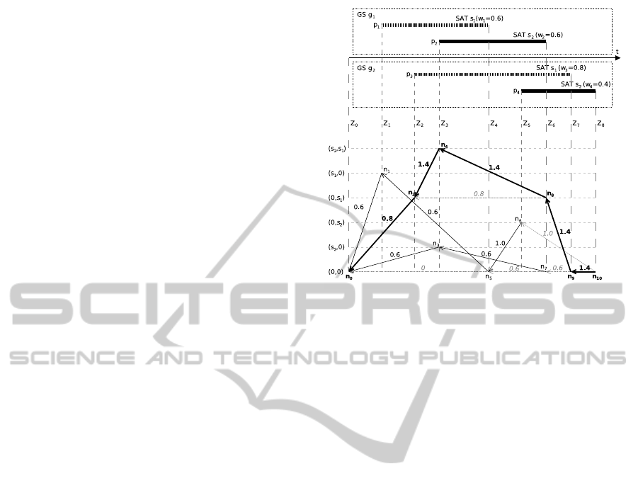
4.1 Graph Generation
This example aims to explain the proposed algorithm
in a MuRRSP simple scenario entailing ground sta-
tions g
1
and g
2
, satellites s
1
and s
2
, and 4 passes (one
for each pair station - satellite). The pass intervals are
represented in Figure 1.
The list of the four passes is P = {p
1
, p
2
, p
3
, p
4
}
which we extend into the set of events {e
1
,e
2
,..., e
8
}:
p
1
= (s
1
,g
1
,t
1
,t
4
,w
1
)

e
1
= (t
1
,+1,s
1
,g
1
,w
1
),
e
2
= (t
4
,−1,s
1
,g
1
,0),
p
2
= (s
2
,g
1
,t
3
,t
6
,w
2
)

e
3
= (t
3
,+1,s
2
,g
1
,w
2
),
e
4
= (t
6
,−1,s
2
,g
1
,0)
p
3
= (s
1
,g
2
,t
2
,t
7
,w
3
)

e
5
= (t
2
,+1,s
1
,g
2
,w
3
),
e
6
= (t
7
,−1,s
1
,g
2
,0),
p
4
= (s
2
,g
2
,t
5
,t
8
,w
4
)

e
7
= (t
5
,+1,s
2
,g
2
,w
4
),
e
8
= (t
8
,−1,s
2
,g
2
,0),
where w
1
= 0.6, w
2
= 0.6, w
3
= 0.8 and w
4
= 0.4.
Figure 1: Graph generation for the Example 1.
We obtain the set E by sorting the events by increas-
ing time, so that:
E = {e
1
,e
5
,e
3
,e
2
,e
7
,e
4
,e
6
,e
8
}. (4.1)
Stage Z
0
: We initialize the algorithm with i =
0,B
−1
=
/
0,n
0
= (0,0),v
0
= (n
0
,
/
0,0) and Z
0
= B
0
=
{n
0
}.
Stage Z
1
: We take the first element in E, which is
e
1
. There is only one node to evaluate in the fron-
tier B
0
, which is n
0
. This node complies with the
conditions in first paragraph of eq. 3.5: (a) there is
no satellite assigned to the ground station indicated in
the event (s(n
0
,g(e
1
)) = s(n
0
,g
1
) = 0), (b) the satel-
lite indicated in the event is not assigned to any other
ground station (s(n
0
,g
′
) 6= s(e
1
) = s
1
∀g
′
), and (c) we
have the edge v
0
= (n
0
,
/
0,0), so that we proceed to
create the new node n
1
.
From the second paragraph of expression 3.5, the
new node has the same values for all its elements
except for the ground station indicated in the event
g(e
1
) = g
1
, which had assigned a zero, and now has
assigned s(e
1
) = s
1
, so that n
1
= (s
1
,0). We also cre-
ate the new edge from the new node (n
1
) to the ex-
amined one (n
0
), with a weight equal to the sum of
the edge from n
0
to
/
0 and the weight of the event
w(e
1
) = w
1
, so that v
1
= (n
1
,n
0
,w
1
).
There are no more nodes to examine in B
0
, so that
Z
1
= {n
1
}, and B
1
= B
0
∪ Z
1
= {n
0
,n
1
}.
Stage Z
2
: The next event in E is e
5
, which is also
a start time event. In this case we evaluate the nodes
in B
1
, which are n
0
and n
1
. Note that n
1
can not be
extended, because s(e
5
) = s(n
1
,g
1
), i.e. the satellite
indicated in the event is already assigned to another
ground station. Note that this avoids the conflict were
OptimalFixedIntervalSatelliteRangeScheduling
405

two ground stations would be tracking the same satel-
lite.
Then we can only extend node n
0
, which follow-
ing the procedure in previous stage yields a new node
n
2
= (0,s
1
), and an edge v
2
= (n
2
,n
0
,w
3
). Then,
Z
2
= {n
2
}, and B
2
= B
1
∪ Z
2
= {n
0
,n
1
,n
2
}.
Stage Z
3
: Also following previous procedure, we
examine n
0
, n
1
and n
2
. Node n
1
is dismissed since
g(e
3
) = g
1
has already assigned s
1
(s(n
1
,g(e
3
)) =
s
1
6= 0).
Extending nodes n
0
and n
2
we create the pairs
n
3
= (s
2
,0),v
3
= (n
3
,n
0
,w
2
) and n
4
= (s
2
,s
1
),v
4
=
(n
4
,n
2
,w
3
+ w
2
), so that Z
3
= {n
3
,n
4
} and B
3
=
{n
0
,n
1
,n
2
,n
3
,n
4
}.
Stage Z
4
: Next event in E is e
4
, which is an end
time event (φ(e
4
) < 0). According to the conditions
in expression 3.7, we only examine the nodes in B
3
which have the satellite s(e
4
) = s
2
assigned to the
ground station g(e
4
) = g
1
, which is only the node
n
1
= (s
1
,0). Note that v
1
= (n
1
,n
0
,w
1
), and also there
is an only node in B
3
which has the same state that
n
1
except for the only change in the ground station
g(e
4
) = g
1
, which has assigned a zero, and this node
is n
0
= (0,0), with v
0
= (n
0
,
/
0,0).
We thus will select one of the two nodes, n
0
or
n
1
, the one with the highest accumulated weight on
its associated vector (v
0
or v
1
). Since the weight of
v
0
is lesser than that of v
1
we select n
1
as the end of
the edge to be created from the new node. We cre-
ate then the new node n
5
= (0, 0) and the new edge
v
5
= (n
5
,n
1
,w
1
). Note that this selection dismisses
unoptimal sub-paths.
As no more nodes from B
3
can be extended, the
set of created nodes is {n
5
}, and the set of deleted
nodes is {n
0
,n
1
}. The new frontier is {B
3
∪ {n
5
}} −
{n
0
,n
1
}, which is B
4
= {n
2
,n
3
,n
4
,n
5
}.
Rest of Stages: Following the same procedures
with the rest of the events we generate the rest of
nodes and edges,
n
0
= (0,0), v
0
= (n
0
,
/
0,0),
n
1
= (s
1
,0), v
1
= (n
1
,n
0
,0.6),
n
2
= (0,s
1
), v
2
= (n
2
,n
0
,0.8),
n
3
= (s
2
,0), v
3
= (n
3
,n
0
,0.6),
n
4
= (s
2
,s
1
), v
4
= (n
4
,n
2
,1.4),
n
5
= (0,0), v
5
= (n
5
,n
1
,0.6),
n
6
= (0,s
2
), v
6
= (n
6
,n
5
,1.0),
n
7
= (0,0), v
7
= (n
7
,n
3
,0.6),
n
8
= (0,s
1
), v
8
= (n
8
,n
4
,1.4),
n
9
= (0,0), v
9
= (n
9
,n
8
,1.4),
n
10
= (0,0), v
10
= (n
10
,n
9
,1.4),
and the stages and frontiers:
Z
0
= {n
0
}, B
0
= {n
0
},
Z
1
= {n
1
}, B
1
= {n
0
,n
1
},
Z
2
= {n
2
}, B
2
= {n
0
,n
1
,n
2
},
Z
3
= {n
3
,n
4
}, B
3
= {n
0
,n
1
,n
2
,n
3
,n
4
},
Z
4
= {n
5
}, B
4
= {n
2
,n
3
,n
4
,n
5
},
Z
5
= {n
6
}, B
5
= {n
2
,n
3
,n
4
,n
5
,n
6
},
Z
6
= {n
7
,n
8
}, B
6
= {n
6
,n
7
,n
8
},
Z
7
= {n
9
}, B
7
= {n
6
,n
9
},
Z
8
= {n
10
}, B
8
= {n
10
}.
We calculate the longest path walking the graph from
the last node: n
10
,n
9
,n
8
,n
4
,n
2
,n
0
. From this set, only
nodes n
2
and n
4
correspond to start time events, and
specifically those from passes p
3
and p
2
.
We show the generated graph in Figure 1, where
we mark the longest path in bold lines. Those edges
which have not been created (but checked for cre-
ation) have been represented as light grey dotted lines.
4.2 Simulation: Practical Case
For this example a scenario consisting of several
ground stations and LEO satellites has been consid-
ered, where the visibility windows of the satellites
over the ground stations generate the passes. The al-
gorithms have been implemented in MATLAB, and
the simulations were run on a virtual machine with a
3 GHz processor and 2 GB RAM.
The greedy algorithm is known to be optimal for
the FI-SiRRSP with no prioritization among passes
(Burrowbridge, 1999; L. Barbulescu, 2004). This
algorithm selects, given a list of passes ordered by
non-descending end time, the next pass which can be
tracked, and mark as unfeasible all the passes in the
list which are conflicting with it. Its worst case com-
plexity is O(N
2
).
However the greedy algorithm is not generally op-
timal for the MuRRSP (nor for the SiRRSP with pri-
orities). A simple example is provided in an scenario
with 3 passes, all mutually conflicting but second with
third. In this case the first one would be selected,
whereas the optimal decision would have been select-
ing second and third ones. For the prioritized case,
consider a scenario with only two conflicting passes
where the second has a higher priority than the first
one.
The selection of the heuristic is crucial for the
performance of the greedy algorithm. Apart from
the end-time ordering heuristic introduced in (Bur-
rowbridge, 1999), we also considered for the simula-
tions the ordering based on the priorities of the passes
(and end-times for passes with equal priority). Note
that neither this heuristic provides an optimal sched-
ule in the FI-SiRRSP with priorities, consider a sce-
ICORES2014-InternationalConferenceonOperationsResearchandEnterpriseSystems
406

0
10
20
30
40
50
60
70
80
90
100
0 500 1000 1500 2000 2500
|P | [passes]
t
SIM
[s]
Optimal
Greedy t
e
i
Greedy w
i
Figure 2: Simulation times for the Example 2.
5
1
1
0
8
.
9
1
7
0
.
3
2
2
8
2
8
8
.
9
3
4
6
.
6
4
0
7
.
2
4
7
1
.
6
5
3
2
.
5
5
9
2
.
4
6
5
8
.
8
7
1
7
.
9
7
7
3
8
2
2
0.5
0.55
0.6
0.65
0.7
0.75
0.8
0.85
0.9
0.95
1
0 500 1000 1500 2000 2500
|P | [passes]
kP
f
k
Σw
· kP
*
k
− 1 Σw
Optimal
Greedy t
e
i
Greedy w
i
Figure 3: Metric ratios for the Example 2.
nario with three passes where first conflicts with sec-
ond, second with third, and the priority of the second
is greater than others’ but smaller than other’s sum.
We run the three algorithms on a scenario with
|G| = 5 stations and |S| = 5 satellites, varying the
size of the scheduling window from 1 to 14 days.
We only use these numbers to show how the dynam-
ics of the problem influence the complexity of the
algorithm. As the number of entities increases, bet-
ter times are clearly foreseeable for the greedy algo-
rithm based on the complexity bounds of the algo-
rithms. Furthermore, passes are given a random pri-
ority w
i
= v
i
/10 : v
i
∼ U[1,10].
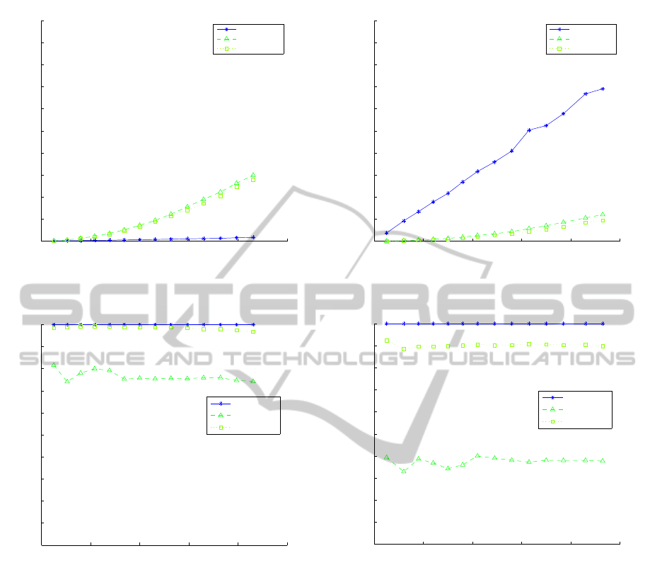
Figure 2 shows the execution time of the three
algorithms versus the number of passes |P| (cor-
responding to the scheduling windows for T =
{1,2,...,14} days. It can be seen that the execution
0
10
20
30
40
50
60
70
80
90
100
0 500 1000 1500 2000 2500
|P | [passes]
t
SIM
[s]
Optimal
Greedy t
e
i
Greedy w
i
Figure 4: Simulation times for the Example 3.
2
1
.
1
5
0
.
7
7
3
.
7
9
7
.
6
1
2
2
.
7
1
4
5
.
7
1
7
2
.
1
2
0
0
.
5
2
2
8
.
5
2
5
7
2
8
7
.
7
3
1
6
.
8
3
5
4
.
7
3
8
3
0.5
0.55
0.6
0.65
0.7
0.75
0.8
0.85
0.9
0.95
1
0 500 1000 1500 2000 2500
|P | [passes]
kP
f
k
Σw
· kP
*
k
− 1 Σw
Optimal
Greedy t
e
i
Greedy w
i
Figure 5: Metric ratios for the Example 3.
time of the optimal algorithm grows linearly with the
number of passes, whereas the greedy algorithms’ do
quadratically. Increasing the number of entities will
imply higher execution times for the optimal algo-
rithm, however still outperforming the times of the
other algorithms for high |P| values.
Figure 3 shows the ratio of the metrics (defined
in expression 2.5) kP
f
k
Σw
· kP
*
k
−1
Σw
, for which the
value of the metric kP
*
k
Σw
of the optimal algorithm
is displayed. Note that the priority-ordering heuristic
achieves near-optimal schedules, but never optimal,
for the studied cases.
4.3 Simulation: Worst Case
This example corresponds to the worst case scenario
for the presented algorithm, wherein all the locations
OptimalFixedIntervalSatelliteRangeScheduling
407

are identical, and so are all the orbits; so that this
case yields the maximum number of conflicts. As for
the previous case, priorities are generated randomly.
Of course this does not correspond to a practical sce-
nario, but will allow to benchmark the worst case be-
haviour of the algorithm.
Simulation times are displayed in Fig. 4, with sim-
ilar considerations as those given for Fig. 2. Note
that whereas the linear coefficient for the execution
time of the optimal algorithm grows, the greedy al-
gorithm reduces its execution time. However, as the
scheduling window extends, the execution time for
the greedy-based algorithms get worse.
Although we provided upper bounds for the com-
plexity of the presented algorithm, it will be relaxed
as the number of conflicts diminishes, or equivalently,
with the dispersion of the locations and orbits. This
can be easily concluded from the way the graph is
constructed, taking into account all the possible com-
binations of tracked passes (see Figs. 2 and 4). The
greedy algorithm improves however its performance
as the number of conflicts rise, as for every pass se-
lection a group of passes can be dismissed, leading
to a shorter execution time. We conjecture that the
increase in the number of conflicts reduces the likeli-
hood of the heuristic algorithms to find a near-optimal
solution (see Figs. 3 and 5).
It is worth reminding that the schedules given by
the greedy algorithm would be optimal for this exam-
ple if the priorities were all the same.
5 CONCLUSIONS
In this paper we have provided the first exact algo-
rithm in polynomial time for the Fixed Interval SRS
problem with a fixed number of ground stations or
satellites, based on the algorithm presented in ref.
(Arkin and Silverberg, 1987) for general scheduling.
Even though the presented algorithm runs in poly-
nomial time, the tractability can be compromised for
cases where the number of ground stations and satel-
lites is high, and locations and orbits are respec-
tively highly correlated. In this sense approaches
toward online scheduling (Papadimitriou and Yan-
nakakis, 1989) should be pursued.
These results for fixed interval scheduling can
be extended to more general cases, through the dis-
cretization of the variable size requests. We are work-
ing on this generalization, as well of in distributed
scheduling approaches.
ACKNOWLEDGEMENTS
This research was performed while the author held
a National Research Council Research Associateship
Award at the Air Force Research Laboratory (AFRL).
We thank Configurable Space Microsystems
Innovations & Applications Center (COSMIAC,
www.cosmiac.org) for the infrastructure support dur-
ing this research.
We thank six anonymous reviewers for their valu-
able comments for improving the manuscript.
REFERENCES
A. W. J. Kolen, J. K. Lenstra, C. H. P. F. C. R. S. Interval
scheduling: A survey.
Arkin, E. M. and Silverberg, E. B. (1987). Scheduling jobs
with fixed start and end times. In Discrete Applied
Mathematics, Vol. 18, pp. 1-8. North-Holland.
Burrowbridge, S. E. (1999). Optimal allocation of satellite
network resources. In Master Thesis. Virginia Poly-
technic and State University.
F. Marinelli, F. Rossi, S. N. S. S. (2005). A lagrangian
heuristic for satellite range scheduling with resource
constraints. In Computers & Operations Research,
Vol. 38, Issue 11, pp. 1572-1583. Elsevier.
H. Jung, M. Tambe, A. B. B. C. (2002). Enabling efficient
conflict resolution in multiple spacecraft missions via
dcsp. In Proceedings of the NASA workshop on plan-
ning and scheduling. NASA.
L. Barbulescu, J. P. Watson, L. D. W. A. E. H. (2004).
Scheduling space-ground communications for the air
force satellite control network. In Journal of Schedul-
ing, Vol. 7, Issue 1, pp. 7-34. Kluwer Academic Pub-
lishers.
M. Y. Kovalyov, C. T. Ng, T. C. E. (2007). Fixed inter-
val scheduling: Models, applications, computational
complexity and algorithms. In European Journal of
Operations Research, Vol. 178, pp. 331-342. Elsevier.
Musser, D. R. (1997). Introspective sorting and selection al-
gorithms. In Software: Practice and Experience, Vol.
27, Issue 8, pp. 983-993. Wiley.
Papadimitriou, C. H. and Yannakakis, M. (1989). Shortest
paths without a map. In Lecture Notes in Computer
Science, Vol. 372, pp. 610-620. Springer.
Vallado, D. A. (2001). Fundamentals of astrodynamics and
applications. Space Technology Library.
Wolfe, W. J. and Sorensen, S. E. (2000). Three schedul-
ing algorithms applied to the earth observing systems
domain. In Management Sience, Vol. 46, No. 1, pp.
148-168. Informs.
ICORES2014-InternationalConferenceonOperationsResearchandEnterpriseSystems
408