Rule-based Classiﬁcation of Visual Field Defects

Enkelejda Kasneci

, Gjergji Kasneci

, Ulrich Schiefer

and Wolfgang Rosenstiel

Department of Computer Engineering, University of T

ubingen, T

ubingen, Germany

Hasso-Plattner-Institute, Potsdam, Germany

Centre for Ophthalmology, Institute for Ophthalmic Research, University of T

ubingen, T

ubingen, Germany

Keywords:

Scotoma, Rule-based, Classiﬁcation, Visual Field, Defect.

Abstract:

The automated recognition of the visual ﬁeld defect type from results of visual ﬁeld testing is crucial for the

adequate diagnosis and treatment of the underlying disease of the visual system. This paper presents a reliable

rule-based classiﬁer that emulates the decision strategies of expert ophthalmologists based on a two-level

approach that combines methods of unsupervised learning.

1 INTRODUCTION

Diseases affecting the optic nerve (e.g., glaucoma),

or the brain (e.g., stroke, trauma, brain injury) may

lead to blind areas or areas of reduced visual percep-

tion in the visual ﬁeld. Such areas, also known as vi-

sual ﬁeld defects (or scotoma), are identiﬁed through

the measurement of the visual ﬁeld, i.e., perimetry.

During a perimetric examination, light stimuli of dif-

ferent luminance levels are projected onto a uniform

background at predeﬁned locations in the visual ﬁeld.

The subject conﬁrms stimulus perception by pressing

a button; no response to a stimulus projection is in-

terpreted as failure to see the stimulus. Visual ﬁeld

defects are areas at which stimuli are not perceived or

only perceived when the stimuli have high light inten-

sity.

Figure 2(a) depicts a perimetric result showing a

central visual ﬁeld defect. Locations of perceived

stimuli are marked by black dots. Rectangles rep-

resent stimuli locations with reduced visual percep-

tion. The darker the rectangle, the lower the sensi-

tivity at that location. The detected location, shape

and size of defects in the visual ﬁeld are hints for the

underlying disease of the visual system. In the clin-

ical routine, the classiﬁcation of the visual ﬁeld de-

fect type from perimetric measurements is performed

manually based on the T

ubingen Scotoma Classiﬁca-

tion Scheme (TSCS), which combines expert know-

how and long-term experience. This scheme distin-

guishes between eight classes of visual ﬁeld defects

as depicted in Figure 1.

The high variability in the manifestation of visual

ﬁeld defect types makes the automated classiﬁcation

of visual ﬁeld defects from perimetric results highly

challenging. Moreover, the measurement data may be

sparse or noisy.

Most prior techniques (Bizios et al., 2007; Boden

et al., 2007; Brigatti et al., 1997; Goldbaum et al.,

1994; Goldbaum et al., 2002; Goldbaum, 2005; Gold-

baum et al., 2009; Henson et al., 1997) have focused

on the automated detection of glaucoma from peri-

metric results, as it is a progressive disease that is

becoming more present due to demographic aging.

Other methods have considered a subset of the vi-

sual ﬁeld defects in terms of the TSCS (Keating et al.,

1993; Mutlukan and Keating, 1994). The extension

and applicability of these methods to the recogni-

tion of other defect types has not been investigated.

Classiﬁcation techniques for the detection of all vi-

sual ﬁeld defect types based on neural networks have

been presented in (Fink, 2004; J

urgens et al., 2001).

These approaches, however, do not report how the

performance of the algorithms varies with decreasing

quality of the data from perimetric results. The main

drawback of methods that are based on neural net-

works is their dependence on the training procedure,

as the overall classiﬁcation performance can be nega-

tively inﬂuenced by missing correlations and noise in

the input data (Bengtsson et al., 2005; Henson et al.,

1997).

In this work we consider all the TSCS types of vi-

sual ﬁeld defects and provide a highly accurate rule-

based classiﬁcation technique that integrates expert

knowledge with parameters that were statistically es-

tablished from a large number of real-world visual

Kasneci E., Kasneci G., Schiefer U. and Rosenstiel W..

Rule-based Classiﬁcation of Visual Field Defects.

DOI: 10.5220/0004746200340042

In Proceedings of the International Conference on Health Informatics (HEALTHINF-2014), pages 34-42

ISBN: 978-989-758-010-9

 2014 SCITEPRESS (Science and Technology Publications, Lda.)

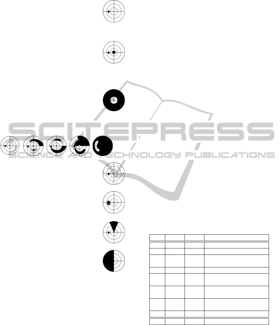
Normal visual ﬁeld: Less than 7 relative de-

fects may occur anywhere in the visual ﬁeld,

but not in the edges of the grid. No defect

clusters besides the physiological blind spot

are visible.

Central scotoma: Defect that occurs within

◦

eccentricity without respecting the verti-

cal or the horizontal meridian. Includes also

the Paracentral scotoma (normal blind spot

position) and the Centrocecal scotoma (ex-

tending from the blind spot towards the cen-

tral area symmetrically above and below the

midline).

Concentric constriction: Visual ﬁeld loss

sparing the central visual ﬁeld.

Glaucoma: Progressive defect that occurs in ﬁve stages

(Aulhorn and Karmeyer, 1977), from relative (left) to

massive absolute defect (right).

Diffuse visual ﬁeld defect: More than 7 rela-

tive defects that are disseminated across the

visual ﬁeld.

Blind spot enlargement: Defect involving at

least two points that are contiguous with the

blind spot.

Sector- oder wedge-shaped defect: Wedge-

shaped defect respecting neither the vertical

nor the horizontal meridian.

Hemianopic: Defect respecting, at least

locally, the vertical meridian.

Others: Defects that cannot be attributed to any of the

above mentioned classes.

Figure 1: T

ubingen Scotoma Classiﬁcation Scheme

(TSCS) (Nevalainen et al., 2007)

ﬁeld examinations. Thus, our method is not neces-

sarily dependent on correlations in the training or in-

put data. In contrast to related methods, our approach

has been evaluated on perimetric results of different

quality levels.

2 INPUT DATA

Perimetric results consisting of 192 concentrically ar-

ranged stimuli locations (e.g., Figure 2(a)) are input

data to our classiﬁcation method. The result con-

cerning the detection of a stimulus location by the

test subject is represented by a stimulus vector s

, y

, dd

), i ∈ {0, . . . , 191}. (x

, y

) represents the

position of the stimulus with x

, y

∈ {−30,···, 30}.

represents the defect depth that is related to the

measured differential luminance sensitivity at loca-

tion (x

, y

). The range of defect values from 0 dB

to over 30 dB is subdivided into 7 intervals, i.e.,

∈ {0, ··· , 6} classes. A perimetric result can be

represented as a matrix of stimuli vectors:

M =













···





191









(1)

The classiﬁcation method was evaluated on 8,868

anonymized visual ﬁeld examination results provided

by the University Eye Hospital T

ubingen. The data

was hand-labeled by expert ophthalmologists. In ad-

dition, a classiﬁcation quality, Q ∈ {2, 3, 4}, repre-

senting the physician’s certainty for the identiﬁcation

of the visual ﬁeld defect, was provided. Q = 4 is the

highest quality level, i.e., the defect type could clearly

be identiﬁed. The distribution of perimetric results

among the defect classes is presented in Table 1.

Table 1: Distribution of defect types in the evaluation

dataset of perimetric results with quality level (Q4-Q2).

Q4 Q3 Q2 Visual ﬁeld defect class

690 1,622 123 C

: Normal visual ﬁeld

16 634 430 C

: Central scotoma

13 111 51 C

: Concentric constric-

tion

125 2,956 999 C

: Glaucoma

1 16 2 C

: Diffuse visual ﬁeld

defects

9 268 153 C

: Blind spot enlarge-

ment

0 19 8 C

: Sector- or wedge-

shaped defect

105 315 202 C

: Hemianopic defect

959 5,941 1,968

3 CLASSIFICATION METHOD

Our method for the recognition of the visual ﬁeld de-

fect type from a perimetric result consists of three

steps:

Rule-basedClassificationofVisualFieldDefects

1. In a ﬁrst step, structures in perimetric exami-

nations, i.e., clusters of stimuli locations with

impaired visual perception, are found. This is

achieved by two methods of unsupervised learn-

ing, namely Hierarchical Agglomerative Clus-

tering (HAC) (Duda et al., 2000) and Self-

Organizing Maps (SOMs) (Kohonen, 1990). In

a two-level approach, SOMs are used to compute

prototype clusters, which are then combined to ﬁ-

nal clusters using HAC. The most decisive beneﬁt

of the SOM-based pre-clustering is noise reduc-

tion (Mangiameli et al., 1996; Henson et al., 1997;

Tafaj et al., 2011a).

2. In the next step, for the original perimetric result

new features are derived from the clusters found

in Step 1, e.g., centroid position, cluster size, aver-

age defect depth of stimuli locations in the cluster,

etc.

3. Finally, ﬁrst-order logic rules check the class

membership of the enriched perimetric result (i.e.,

with the above features). The rules have been

designed in close collaboration with expert oph-

thalmologists. Uncertain decision parameters

(e.g., decision thresholds) have been optimized by

means of correlation analysis.

Step 1: Clustering for the Feature

Enrichment of Perimetric Results

Pre-clustering through Self-Organizing Maps: A

Self-Organizing Map (SOM) is an unsupervised

learning method introduced by Kohonen (Kohonen,

1990). In a SOM network, the N-dimensional in-

put data is mapped to a lower dimensional arrange-

ment (grid) of neurons, such that the topological or-

der is maintained (Kohonen, 1990). Thus, adjacent

units map to similar data points. The particularity

of a SOM is that it can be used at the same time for

both the reduction of data complexity (by clustering)

and the nonlinear projection onto a lower-dimensional

space (Kaski, 1997). Each neuron, also called unit, is

assigned a reference vector m

containing the synaptic

weights. These reference vectors are initialized prior

to the SOM training, usually randomly. During train-

ing, the reference vectors of the map units are iter-

atively adapted to ﬁt the input data best. Given the

input data point x, for each unit, the distance between

its reference vector and x is computed. The Kohonen

unit c with the minimum distance to x (usually the

Euclidean metric is used) is the winner neuron, also

called Best Matching Unit, BMU, Equation 2:

c = c(x) = argmin

{

x −m

} (2)

Thus, the BMU determines the spatial location

of a topological neighborhood of excited neurons,

thereby providing the basis for cooperation among

neighboring neurons. In each new iteration step t + 1,

the reference vectors are adapted to the input from the

previous iteration step, x(t), according to the gradient

descent rule in Equation 3:

(t + 1) = m

(t) + α(t)h

[x(t) −m

(t)] (3)

α(t) represents the learning rate over time (which

typically decreases with learning progress), whereas

represents the neighborhood kernel around the

BMU c.

Hierarchical Agglomerative Clustering: In HAC

clusters of points are constructed in a bottom-up man-

ner; starting with each point as a singleton clus-

ter, clusters that are close to each other, according

to a predeﬁned similarity or distance measure, e.g.,

the Euclidean distance, are merged iteratively until a

single, all-encompassing cluster remains (Jain et al.,

1999; Tan et al., 2005). We use HAC with centroid-

linkage on top of the SOM-based pre-clustering of

stimuli locations to derive coherent defect clusters.

Centroid-linkage clustering deﬁnes the cluster dis-

tance as the distance between their centroids (Flach,

2012). The goal of every merge step is to ﬁnd and

merge a pair of clusters c

, c

that minimize the link-

age function L

centroid

, c

centroid

, c

) = D(µ

, µ

) (4)

The SOM-based clustering approach has several

advantages over other popular alternatives, such as k-

means or expectation-maximization-based methods.

Such methods require that the number of clusters

is known in advance. In our scenario, we have no

prior knowledge on the number of clusters. In the

SOM approach, the only parameter that is decisive

for the number of clusters is an empirically estab-

lished threshold on the distance of neighboring neu-

rons. That is, neighboring neurons with a distance

greater than the threshold belong to different clus-

ters. While several ﬂat-clustering algorithms can be

adapted to take such a threshold into account, they

often face the problem of unstable results in the pres-

ence of noise. In fact, noise is the most difﬁcult aspect

to deal with in the scenario of clustering stimuli loca-

tions.

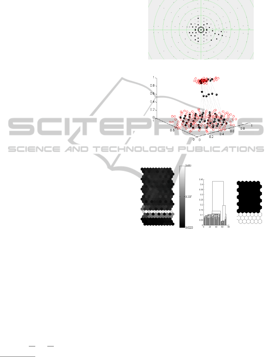
Figure 2 illustrates how this two-level approach

was used for the analysis of visual ﬁeld defects in

perimetric examination results. Figure 2(a) depicts a

perimetric examination result showing a central visual

ﬁeld defect. A SOM grid (12 ×6 units) was trained

on the normalized perimetric data from Figure 2(a)

HEALTHINF2014-InternationalConferenceonHealthInformatics

based on the Matlab SOM Toolbox

. Figure 2(b)

shows the mapping of the SOM units (represented by

black circles) on the normalized perimetric data. Note

that a 3-dimensional representation has been used for

the sake of better visualization. In this example, the

visual ﬁeld defect and the intact area of the visual

ﬁeld form well-separated clusters. Figure 2(c) shows

a so-called U-Matrix for the SOM trained in Fig-

ure 2(b) visualizing the Euclidean distances between

reference vectors of neighboring units (black repre-

sents small Euclidean distance). As is can be seen in

Figure 2(c), a bright set of cells separates two dark

areas that correspond to the clusters in the perimetric

result. Note that separating the clusters of the SOM

from Figure 2(b) according to the corresponding U-

Matrix is straight-forward for the presented example,

which was chosen for the sake of a comprehensible

demonstration of the method. However, note that in

general, the U-Matrix may suggest multiple clusters

with non-obvious boundaries between them. For such

cases further analysis is needed to separate the clus-

ters. Therefore, we apply HAC on top of the SOM

results to separate clusters based on their hierarchical

dependencies derived from the centroid-linkage strat-

egy. This was also done to detect the clusters of units

on the SOM from Figure 2(c). The corresponding

dendrogram and the clustering result are presented in

Figure 2(d).

Step 2: Feature Enrichment

The features of the clusters derived in Step 1 (e.g.,

cluster centroid, cluster size, average defect depth of

stimuli locations in a cluster, etc.) are used to enrich

the original perimetric result. The enriched feature

vector of a perimetric result is x ∈ X contains the

following features:

• the set M of 192 three-dimensional vectors repre-

senting the stimuli (see Equation 1)

• the number n

of defects in the perimetric exami-

nation result

• the number n

of clusters derived by the SOM-

based clustering

• the set of cluster means {µ

, ..., µ

}

• the set of cluster sizes {S

, ..., S

}

• the set of the numbers of stimuli locations in each

cluster {sc

, ..., sc

}

• the set containing the average defect depth in each

cluster {dd

, ..., dd

}

Matlab SOM Toolbox, http://www.cis.hut.ﬁ/projects/

somtoolbox/

(a) Perimetric result showing a central visual ﬁeld

defect

(b) The normalized perimetric data from (a) (red

circles) and a mapped SOM with a lattice of 12x6

units (black circles)

the distances between

neighboring units of the

SOM from (b)

(d) Dendrogram and clusters

resulting from HAC with

centroid-linkage on the SOM

from (b)

Figure 2: An example of SOM usage for clustering perimet-

ric results.

Such an enriched perimetric result becomes the in-

put of the classiﬁer in Step 3, by which it is mapped

to one of the eight visual ﬁeld defect classes depicted

in Figure 1.

Step 3: Recognition of Visual Field Defect

Types

The classiﬁer has been designed as a function

f : X → C , C = {C

, . . . ,C

}, that maps an input

x ∈ X to one of the 8 classes in C in a way that is

similar to how an expert ophthalmologist would de-

cide, namely based on rules derived from frequently

Rule-basedClassificationofVisualFieldDefects

occurring observations. Hence, the classiﬁcation

method consists of a collection of rule-based binary

classiﬁers that operate based on a one-versus-all

scheme. For each of the 8 classes, a ﬁrst-order logic

rule has been manually assembled by considering

decision rules used by ophthalmologists and also

by empirically analyzing a hand-labeled data set

of perimetric results of quality levels 3 and 4, see

Table 1. This data set was recommended by an expert

ophthalmologist and included 20 representatives of

each scotoma class, except for the classes C

and C

which were represented by 10 perimetric results each.

In order to identify appropriate values for some of the

input features (i.e., for values that are prone to uncer-

tainty), a correlation analysis was run on this data set

with the goal of increasing the accuracy of the sco-

toma classiﬁer. To this end, the Matthews Correlation

Coefﬁcient, MCC, was computed on the number of

true positives (TP), true negatives (TN), false posi-

tives (FP), and false negatives (FN) for a given class:

MCC =

T P×TN−FP×FN

√

(T P+FP)(T P+FN)(T N+FP)(T N+FN)

(Baldi

et al., 2000). The characterization of each class is

based on the TSCS from Figure 1.

Normal Visual Field (C

). The normal visual ﬁeld

is characterized by only one defect cluster that corre-

sponds to the physiological blind spot and few spo-

radic defects that occur due to the patient’s inatten-

tion. The correlation analysis on the data revealed a

maximum number of 10 defects. Note that this thresh-

old is in accordance with typical thresholds used by

expert ophthalmologists, which range between 8 and

11. This number includes the failed stimuli loca-

tions within the blind spot cluster c

blindspot

with cen-

troid µ

blindspot

and size S

blindspot

, and few sporadic de-

fects. The values µ

blindspot

and S

blindspot

stem from the

TSCS.

≤ 10 ∧ n

= 1 ∧ µ ≈ µ

blindspot

∧

S ≈S

blindspot

) →C

(5)

Central Scotoma (C

). A central scotoma is char-

acterized by absolute or relative defects that do not

respect the vertical or horizontal meridian in the cen-

tral visual ﬁeld. A perimetric result is assigned to this

class if it fulﬁlls the rule (RC ∨RCC) →C

, where RC

and RCC are deﬁned in the Formulas 6 and 7, respec-

tively.

The RC part of the rule stems entirely from expert

knowledge: All 13 stimuli locations within 2

◦

eccen-

tricity are checked; if more than 50% of these loca-

tions, i.e., more than 6, are defects, the presence of a

central scotoma is assumed.

[RC] :

∑

∈M

(

, y

)

≤ 2)(dd

≥ 1)) ≥ 6 (6)

RCC stems also to a large extent from expert

knowledge: A paracentral scotoma is assumed when-

ever there exists a central cluster of defects with cen-

troid within 10

◦

eccentricity, containing more than 5

stimuli. The minimum number of stimuli locations

within the central cluster was derived from correla-

tion analysis (i.e., MCC analysis) on the data. The

value 5 was revealed as a reliable threshold.

[RCC] : ∃c

≤ 10 ∧ sc

≥ 5 ∧ dd

≥ 3 (7)

Concentric Constriction (C

). This defect type is

manifested by an intact central visual ﬁeld and a pe-

ripheral ﬁeld constriction. Thus, we consider a central

(within 15

◦

eccentricity) and a peripheral defect clus-

ter and check their positions. In addition, the average

defect depths in the clusters are compared. The de-

fect depth in the peripheral defect cluster is expected

to be at least 1.3 times larger than the defect depth in

the central cluster. The values 15 and 1.3 were estab-

lished by means of MCC analysis on the data.

(∃c

, c

: µ

≈ (0, 0) ∧ ∀s

∈ c



, y

)



≤ 15

∧ µ

≈ (0, 0) ∧ dd

≥ dd

∗1.3) →C

(8)

Glaucoma (C

). This class is characterized by

arcuate-shaped defects. However, the perimetric re-

sults for this class only rarely showed well-separated

defect clusters as depicted in the schematic view of

Figure 1. In reality, the defect clusters were often

distorted. Furthermore, the ﬁve stages of glaucoma

reveal different cluster shapes. A perimetric exami-

nation is classiﬁed as glaucomatous if there exists a

cluster with at least 15 defects spanning over the right

and left hemiﬁeld according to the rule in Equation 9.

While a minimum average defect depth of dd

= 3

is a typical value observed by experts, the remaining

thresholds were established by means of MCC analy-

sis.

(∃c

: sc

≥ 15 ∧ dd

≥ 3 ∧

∃s

, s

∈ c

: x

> 10 ∧ x

< −10) →C

(9)

Diffuse Visual Field Defects (C

). These are de-

fects that are spread across the visual ﬁeld, see Fig-

ure 1. Clustering typically yields one large cluster

encompassing more than half of the visual ﬁeld (i.e.,

≥0.5*VF). Experts also expect to observe an average

defect depth of at least 2 in this cluster.

(∃c

: S

≥ 0.5 ∗V F ∧ dd

≥ 2) →C

(10)

HEALTHINF2014-InternationalConferenceonHealthInformatics

Blind Spot Enlargement (C

) These are defects

that occur due to the enlargement of the blind spot.

Such cases are typically assumed when there is a de-

fect cluster close to the blind spot area, for which the

centroid or the size does not correspond to the cen-

troid or the size of the normal physiological blind spot

cluster. The following is a decision rule used by ex-

pert ophthalmologists for this class of defects.



∃c

: µ

6= µ

blindspot

∨ S > S

blindspot



→C

(11)

Sector- or Wedge-shaped Defects (C

). These are

defect areas that are wedge-shaped. A perimetric re-

sult is assigned to this class, if there is a defect cluster

with the following features: (i) it contains more than 8

defect stimuli, (ii) it is not the blind spot, and (iii) the

angle between the sides of the wedge-shaped cluster

and l

) is between 30

◦

and 90

◦

. The values for the

minimum number of defect stimuli in (i) and the min-

imum average defect depth in (ii) were established by

means of MCC analysis. The angle between the clus-

ter sides stems from expert knowledge.

(∃c

: µ

6= µ

blindspot

∧ S

6= S

blindspot

∧ sc

≥ 8 ∧

≥ 2 ∧ 30 ≤ ∠(l

), l

)) ≤ 90) →C

(12)

Hemianopic Defect (C

). These defects expand

over one hemiﬁeld and respect the vertical meridian

of the visual ﬁeld. The corresponding perimetric

results are typically characterized by an impaired left

or right visual ﬁeld side, where most of the stimuli

were not recognized. The other half of the visual

ﬁeld is intact, except for the blind spot area and few

relative or absolute defects, e.g., due to patient’s

inattention. To detect this defect type, the algorithm

counts the number of defects in each half of the visual

ﬁeld. Correlation analysis on the data, by means of

MCC, revealed that a left-sided hemianopic defect is

found, if at least 60% of the stimuli locations of the

left side (i.e., with x coordinate x ≤ 0) of the visual

ﬁeld are absolute defects (i.e., stimuli locations with

defect depth dd ≥ 3). The threshold 3 for the defect

depth of a stimulus is based on expert knowledge.

The right side of the visual ﬁeld is considered intact,

if there are less than 10% of relative defects (i.e.,

stimuli locations with defect depth dd ≤2). The rule

for the detection of the left-sided hemianopic defect

is deﬁned by RHL in Formula 13. The detection

of a right-sided hemianopic defect is deﬁned by

RHR in the Formula 14 and is symmetric to RHL.

In summary, a perimetric examination result is

assigned to this defect class if it fulﬁlls the rule

(RHL ∨RHR) →C

[RHL] :

∑

∈M

((x

≤ 0)(dd

≥ 3))

∑

∈M

≤ 0)

≥ 0.6 ∧

∑

∈M

((x

> 0)(dd

≤ 2))

∑

∈M

> 0)

≤ 0.1 (13)

[RHR] :

∑

∈M

((x

≥ 0)(dd

≥ 3))

∑

∈M

≥ 0)

≥ 0.6 ∧

∑

∈M

((x

< 0)(dd

≤ 2))

∑

∈M

< 0)

≤ 0.1 (14)

Note that in general more than one of the presented

decision rules may ﬁre for the same input. Under

the assumption that each perimetric examination re-

sult belongs to one and only one defect class, we iter-

ate through the rules in the order they were introduced

and the class corresponding to the ﬁrst rule that ﬁres.

4 EXPERIMENTAL RESULTS

The presented algorithm was evaluated on all 8, 848

perimetric examination results of quality levels 4, 3,

and 2 from Table 1, in a one-against-all scheme. The

classiﬁcation performance was measured by means of

accuracy (ACC) and speciﬁcity (SP). The evaluation

results of the classiﬁcation method are presented in

Table 2. For each scotoma class and the correspond-

ing quality level, the ACC and SP values are reported.

Furthermore, weighted average values for ACC and

SP are shown per defect type, as well as for the entire

data set.

The overall classiﬁcation ACC and SP of the pre-

sented rule-based classiﬁcation method were 83% and

85%, respectively. For examination results of qual-

ity level 4, the average (weighted) ACC and SP val-

ues were 92% and 98%, respectively. Considering

the three defect classes with the largest number of in-

stances, namely normal visual ﬁeld, glaucoma, and

hemianopic defect, the algorithm shows very good

performance, i.e., ACC and SP values of above 90%.

With decreasing data quality (from examination

results of quality level 4 to examination results of

quality level 2), which corresponds to increasing un-

certainty in classiﬁcation by the ophthalmologists, we

found that the performance of our algorithm also de-

creases, see Table 2. For examination results of qual-

ity levels 3 and 2, there was a decrease in the average

ACC and SP values to 87% and 85% (for quality level

3) and 79% and 78% (for quality level 2), respec-

tively. This effect could be observed for each scotoma

class. The main reason for this effect is the high diver-

sity of manifestations of a scotoma type, which may

Rule-basedClassificationofVisualFieldDefects

Table 2: Evaluation of the accuracy (ACC) and speciﬁcity (SP) of the rule-based classiﬁer on 8, 848 hand-labeled perimetric

examination results.

Weighted avg. Quality 4 Quality 3 Quality 2

Visual ﬁeld defect class ACC

(%)

ACC

(%)

ACC

(%)

ACC

(%)

: Normal visual ﬁeld 91 97 91 98 91 97 90 92

: Central scotoma 83 82 91 91 86 85 80 78

: Concentric constriction 88 89 97 98 89 90 84 85

: Glaucoma 76 78 93 95 77 79 74 73

: Diffuse visual ﬁeld defects 88 88 95 95 88 88 86 86

: Blind spot enlargement 83 84 94 95 85 85 81 82

: Sector- or wedge-shaped defect 88 88 97 97 88 89 87 87

: Hemianopic defect 91 92 97 98 90 91 89 90

Overall 83 85 92 98 87 85 79 78

lead to uncertainty in the classiﬁcation result by the

physician or a miss-classiﬁcation by the algorithm.

The largest loss in ACC (i.e., from 93% for data

of quality level 4 to 74% for data of quality level

2) is found in the recognition of glaucoma. Indeed,

the recognition of glaucoma is considered particularly

challenging (Nouri-Mahdavi et al., 2011), mainly be-

cause of its manifestation in 5 Aulhorn-stages, as de-

picted schematically in Figure 1. In the clinical rou-

tine, the classiﬁcation of glaucoma is not only based

on the perimetric result, but also under considera-

tion of patient-related features, such as the intraocular

pressure. Such features, however, are often difﬁcult

to quantify and were thus not considered in our rule-

based classiﬁcation method.

In some cases, especially for data of low quality,

(e.g., quality level 2) more than one of the presented

decision rules might ﬁre. Under the assumption that

each perimetric examination result belongs to one and

only one defect class, the presented rule iteration or-

der interferes with the classiﬁcation performance.

Comparison to Related Work

The accuracy achieved by our method regarding the

detection of glaucoma varied from 74% (for data of

quality level 2) to 93% (for data of quality level 4), see

Table 2. The overall weighted average accuracy for

glaucoma recognition was 76%, which is well in line

with other approaches (Boden et al., 2007; Brigatti

et al., 1997; Goldbaum, 2005; Goldbaum et al., 2009;

Goldbaum et al., 2002; Goldbaum et al., 1994; Hen-

son et al., 1996; Mutlukan and Keating, 1994). How-

ever, note that these approaches were evaluated on

relatively small data sets consisting of a few hun-

dred perimetric examination results, whereas our al-

gorithm was evaluated on 4,080 perimetric results of

glaucomatous visual ﬁeld defect cases.

An approach that has considered a larger subset of

visual ﬁeld defect classes was presented in (Keating

et al., 1993). The achieved accuracy reported there

varied from 74% to 96% on simulated perimetric re-

sults of the following defect types: (1) central vi-

sual ﬁeld defects, (2) concentric constriction, and (3)

hemianopic defects. Our algorithm outperforms this

approach for all the mentioned defect types and all

data quality levels.

In comparison to the classiﬁcation accuracy of

80% that was achieved by (Fink, 2004), where a

Hopﬁeld-attractor network was used to recognize the

visual ﬁeld defect classes, our algorithm performs

better when considering the overall accuracy on data

of quality levels 4 and 3. For data of quality level

2, our approach yields similar accuracy results as the

approach of (Fink, 2004).

In comparison to the approach presented in

urgens et al., 2001) that achieves a classiﬁcation

accuracy of 95%, our algorithm shows similar perfor-

mance on data of quality level 4, where about 1,000

perimetric results were classiﬁed. It is important

to note that it is unclear how the above approaches

would have performed on large data sets of varying

quality levels.

In summary, the main advantage of our rule-based

scotoma classiﬁer is the integration of expert knowl-

edge into the automated classiﬁcation method. Fur-

thermore, the rules can be easily adapted and new fea-

tures can be included.

5 CONCLUSIONS

We presented a rule-based classiﬁcation method for

the automated recognition of the visual ﬁeld defect

types from visual ﬁeld measurements. This approach

was evaluated on a large set of visual ﬁeld measure-

ments of different quality levels and showed a high

HEALTHINF2014-InternationalConferenceonHealthInformatics

classiﬁcation accuracy. The presented method can

also be used beyond the classiﬁcation purpose. More

speciﬁcally, the two-level approach can be employed

to automatically extract areas of reduced perception

in the visual ﬁeld assessed with methods other than

perimetry, e.g., with EFOV (Tafaj et al., 2013), which

measures the visual exploration capability of a subject

based on the online analysis of eye movements (Tafaj

et al., 2012). Besides its usage in local diagnostic pro-

cesses, e.g., assisting the clinical routine, the method

could also be used in tele-medicine. Further improve-

ments of the presented algorithm include: (1) the re-

ﬁnement of the decision rules and the investigation

of further features, such as features related to the pa-

tient’s general health condition, with the focus on the

glaucoma defect type, (2) the development of a user-

friendly interface for individual threshold adaptation,

and (3) integration with other software tools for vision

research, such as Vishnoo (Tafaj et al., 2011b).

REFERENCES

Aulhorn, E. and Karmeyer, H. (1977). Frequency distribu-

tion in early glaucomatous visual ﬁeld defects. Doc-

umenta Ophthalmologica Proceedings Series, 14:75–

83.

Baldi, P., Brunak, S., Chauvin, Y., Andersen, C. A. F., and

Nielsen, H. (2000). Assessing the accuracy of predic-

tion algorithms for classiﬁcation: an overview. Bioin-

formatics, 16(5):412–424.

Bengtsson, B., Bizios, D., and Heijl, A. (2005). Effects

of input data on the performance of a neural net-

work in distinguishing normal and glaucomatous vi-

sual ﬁelds. Investigative Ophthalmology & Visual Sci-

ence, 46(10):3730–3736.

Bizios, D., Heijl, A., and Bengtsson, B. (2007). Trained

artiﬁcial neural network for glaucoma diagnosis using

visual ﬁeld data: a comparison with conventional al-

gorithms. Journal of Glaucoma, 16(1):20–28.

Boden, C., Chan, K., Sample, P. A., Hao, J., Lee, T.,

Zangwill, L. M., Weinreb, R. N., and Goldbaum,

M. H. (2007). Assessing Visual Field Clustering

Schemes Using Machine Learning Classiﬁers in Stan-

dard Perimetry. Investigative Ophthalmology & Visual

Science, 48(12):5582–5590.

Brigatti, L., Nouri-Mahdavi, K., Weitzmann, M., and Capri-

oli, J. (1997). Automatic Detection of Glaucoma-

tous Visual Field Progression with Neural Networks.

Archives of Ophthalmology, 115(6):725–728.

Duda, R. O., Hart, P. E., and Stork, D. G. (2000). Pat-

tern Classiﬁcation (2nd Edition). Wiley-Interscience,

2 edition.

Fink, W. (2004). Neural attractor network for application

in visual ﬁeld data classiﬁcation. Physics in Medicine

and Biology, 49(13):2799–2809.

Flach, P. (2012). Machine Learning: The art and science of

algorithms that make sense of data. Cambridge Uni-

versity Press.

Goldbaum, M. H. (2005). Unsupervised learning with in-

dependent component analysis can identify patterns of

glaucomatous visual ﬁeld defects. Transactions of the

Americal Ophthalmological Society, 103:270–280.

Goldbaum, M. H., Jang, G. J., Bowd, C., Hao, J., Zangwill,

L. M., Liebmann, J., Girkin, C., Jung, T. P., Wein-

reb, R. N., and Sample, P. A. (2009). Patterns of

glaucomatous visual ﬁeld loss in SITA ﬁelds automat-

ically identiﬁed using independent component analy-

sis. Transactions of the Americal Ophthalmological

Society, 107:136–144.

Goldbaum, M. H., Sample, P. A., Chan, K., Williams, J.,

Lee, T. W., Blumenthal, E., Girkin, C. A., Zangwill,

L. M., Bowd, C., Sejnowski, T., and Weinreb, R. N.

(2002). Comparing machine learning classiﬁers for di-

agnosing glaucoma from standard automated perime-

try. Investigative Ophthalmology & Visual Science,

43(1):162–169.

Goldbaum, M. H., Sample, P. A., White, H., Colt, B.,

Raphaelian, P., Fechtner, R. D., and Weinreb, R. N.

(1994). Interpretation of automated perimetry for

glaucoma by neural network. Investigative Ophthal-

mololgy & Visual Science, 35(9):3362–3373.

Henson, D. B., Spenceley, S. E., and Bull, D. R. (1996).

Spatial classiﬁcation of glaucomatous visual ﬁeld

loss. British Journal of Ophthalmology, 80(6):526–

531.

Henson, D. B., Spenceley, S. E., and Bull, D. R. (1997).

Artiﬁcial neural network analysis of noisy visual ﬁeld

data in glaucoma. Artiﬁcial Intelligence in Medicine,

10(2):99–113.

Jain, A. K., Murty, M. N., and Flynn, P. J. (1999). Data

clustering: a review. ACM Computing Surveys,

31(3):264–323.

urgens, C., Koch, T., Burth, R., Schiefer, U., and Zell, A.

(2001). Classiﬁcation of perimetric results and reduc-

tion of number of test locations using artiﬁcial neural

networks [arvo abstract nr. 4539]. Investigative Oph-

thalmology & Visual Science, 42(4):846.

Kaski, S. (1997). Data exploration using self-organizing

maps. In Acta Polytechnica Scandinavica: Mathe-

matics, Computing and Management in Engineering

Series No 82.

Keating, D., Mutlukan, E., Evans, A., McGarvie, J., and

Damato, B. (1993). A back propagation neural net-

work for the classiﬁcation of visual ﬁeld data. Physics

in Medicine and Biology, 38(9):1263.

Kohonen, T. (1990). The self-organizing map. Proceedings

of the IEEE, 78(9):1464–1480.

Mangiameli, P., Chen, S. K., and West, D. (1996). A com-

parison of som neural network and hierarchical clus-

tering methods. European Journal of Operational Re-

search, 93(2):402–417.

Mutlukan, E. and Keating, D. (1994). Visual ﬁeld interpre-

tation with a personal computer based neural network.

Eye, 8(3):321–323.

Nevalainen, J., Krapp, E., Paetzold, J., Mildenberger, I.,

Besch, D., Vonthein, R., Keltner, J. L., Johnson, C. A.,

Rule-basedClassificationofVisualFieldDefects

and Schiefer, U. (2007). Visual ﬁeld defects in acute

optic neuritis - distribution of different types of defect

pattern, assessed with threshold-related supraliminal

perimetry, ensuring high spatial resolution. Graefe’s

Arch Clin Exp Ophthalmol, 246(4):599–607.

Nouri-Mahdavi, K., Nassiri, N., Giangiacomo, A., and

Caprioli, J. (2011). Detection of visual ﬁeld progres-

sion in glaucoma with standard achromatic perime-

try: A review and practical implications. Graefe’s

Archive for Clinical and Experimental Ophthalmol-

ogy, 249(11):1593–1616.

Tafaj, E., Dietzsch, J., Bogdan, M., Schiefer, U., and Rosen-

stiel, W. (2011a). Reliable classiﬁcatin of visual ﬁeld

defects in automated perimetry using clustering. In

Proceedings of the 8th IASTED International Confer-

ence on Biomedical Engineering, BIOMED ’11.

Tafaj, E., Hempel, S., Heister, M., Aehling, K., Schaef-

fel, F., Dietzsch, J., Rosenstiel, W., and Schiefer, U.

(2013). A New Method for Assessing the Exploratory

Field of View (EFOV). In Stacey, D., Sol-Casals, J.,

Fred, A. L. N., and Gamboa, H., editors, HEALTHINF

2012, pages 5–11. SciTePress.

Tafaj, E., Kasneci, G., Rosenstiel, W., and Bogdan, M.

(2012). Bayesian online clustering of eye movement

data. In Proceedings of the Symposium on Eye Track-

ing Research and Applications, ETRA ’12, pages

285–288, New York, NY, USA. ACM.

Tafaj, E., K

ubler, T., Peter, J., Schiefer, U., Bogdan, M.,

and Rosenstiel, W. (2011b). Vishnoo - an open-

source software for vision research. In Proceedings of

the 24

IEEE International Symposium on Computer-

Based Medical Systems, CBMS’ 11, pages 1–6. IEEE.

Tan, P. N., Steinbach, M., and Kumar, V. (2005). Introduc-

tion to Data Mining. Addison Wesley.

HEALTHINF2014-InternationalConferenceonHealthInformatics