Hierarchical Bayesian Modelling of Visual Attention

Jinhua Xu

Department of Computer Science and Technology, East China Normal University,

500 Dongchuan Road, Shanghai 200241, China

Keywords:

Visual Attention, Visual Saliency, Bayesian Modeling, Object Localization.

Abstract:

The brain employs interacting bottom-up and top-down processes to speed up searching and recognizing visual

targets relevant to speciﬁc behavioral tasks. In this paper, we proposed a Bayesian model of visual attention

that optimally integrates top-down, goal-driven attention and bottom-up, stimulus-driven visual saliency. In

this approach, we formulated a multi-scale hierarchical model of objects in natural contexts, where the com-

puting nodes at the higher levels have lower resolutions and larger sizes than the nodes at the lower levels, and

provide local contexts for the nodes at the lower levels. The conditional probability of a visual variable given

its context is calculated in an efﬁcient way. The model entails several existing models of visual attention as

its special cases. We tested this model as a predictor of human ﬁxations in free-viewing and object searching

tasks in natural scenes and found that the model performed very well.

1 INTRODUCTION

Human and many other animals have a remarkable

ability to interpret complex scenes in real time, de-

spite the limited information-processing speed of the

neuronal hardware available for this task. Intermedi-

ate and higher visual processes appear to select a sub-

set of the incoming sensory information for further

processing. The most important function of selective

visual attention is to direct our gaze rapidly towards

objects of interests in our visual environment. There

are two major categories of factors that drive atten-

tion: bottom-up (BU) factors and top-down (TD) fac-

tors. Bottom-up factors are derived solely from the in-

coming visual stimuli. Regions of interest that attract

our attention in a bottom-up way are deemed salient

and the visual features for this selection must be suf-

ﬁciently discriminative with respect to the surround-

ing features. On the other hand, top-down attention is

driven by cognitive factors such as knowledge, expec-

tations, and current goals (Borji and Itti, 2013).

Computational models of visual attention have

been extensively researched (see (Frintrop et al.,

2010; Toet, 2011) for reviews). Over the past

decade, many different algorithms have been pro-

posed to model bottom-up visual saliency. They can

be broadly classiﬁed as biologically-based (Itti et al.,

1998), purely computational, or a combination of

both(Bruce and Tsotsos, 2009). In Itti et al’s model

(Itti et al., 1998), a measure of saliency is computed

based on the relative difference between a target and

its surround along a set of feature dimensions (i.e.,

color, intensity, orientation, and motion). Several sta-

tistical models of visual saliency have also been de-

veloped (Bruce and Tsotsos, 2009; Zhang et al., 2008;

Gao and Vasconcelos, 2009; Itti and Baldi, 2009). In

these models, a set of statistics or probability distri-

butions (PDs) of visual variables are computed from

either the scene the subject is viewing or a set of

natural scenes, and a variety of measures of visual

saliency are deﬁned on these statistics or PDs, includ-

ing self-information (Bruce and Tsotsos, 2009; Zhang

et al., 2008), discriminant power (Gao and Vasconce-

los, 2009), Bayesian surprise (Itti and Baldi, 2009).

For top-downvisual attention, three major sources

of top-down inﬂuences have been explored, such as

global scene context (Torralba et al., 2006; Peters

and Itti, 2007), object features (appearance) (Kanan

et al., 2009; Gao et al., 2009; Ehinger et al., 2009;

Elazary and Itti, 2010; Rao et al., 2002; Lee et al.,

2002), and task demands (Triesch et al., 2003; Naval-

pakkam and Itti, 2005). In the contextual guidance

model (Torralba et al., 2006), local features, global

features (scene gist), and object locations were inte-

grated, and visual saliency was deﬁned by the prob-

ability of the local features in the scene based on

the scene gist. The gist was used to select relevant

image regions for exploration. In classical search

347

Xu J..

Hierarchical Bayesian Modelling of Visual Attention.

DOI: 10.5220/0004731303470358

In Proceedings of the 9th International Conference on Computer Vision Theory and Applications (VISAPP-2014), pages 347-358

ISBN: 978-989-758-003-1

 2014 SCITEPRESS (Science and Technology Publications, Lda.)

tasks, target features are a ubiquitous source of atten-

tion guidance (Einhauser et al., 2008). For complex

target objects in natural scenes, there are other fea-

tures that can drive visual attention. In (Kanan et al.,

2009), an appearance-based saliency model was de-

rived in a Bayesian framework. Responses of ﬁlters

derived from natural images using independent com-

ponent analysis (ICA) were used as the features. In

(Rao et al., 2002), targets and scenes were represented

as responses from oriented spatio-chromatic ﬁlters at

multiple scales, and saliency maps were computed

based on the similarity between a top-downiconic tar-

get representation and the bottom-up scene represen-

tation.

A prevailing view is that bottom-up and top-down

attention is combined to direct our attentional behav-

ior. An integration method should be able to ex-

plain when and how to attend to a top-down visual

item or skip it for the sake of a bottom-up salient

cue (Borji and Itti, 2013). In (Ehinger et al., 2009),

computational models of search guidance from three

sources, including bottom-up saliency, visual features

of target appearance, and scene context, were investi-

gated and combined by simple multiplication of three

components. In (Zelinsky et al., 2006), the pro-

portions of BU and TD components in a saliency-

based model were manipulated to investigate top-

down and bottom-up information in the guidance of

human search behavior. In (Navalpakkam and Itti,

2007), the top-down component, derived from accu-

mulated statistical knowledge of the visual features

of the desired target and background clutter, was used

to optimally tune the bottom-up maps such that the

speed of target detection is maximized.

A hierarchical Bayesian inference model for early

visual processing was proposed in (Lee and Mum-

ford, 2003). In this framework, the recurrent feed-

forward/feedback loops in the cortex serve to inte-

grate top-down contextual priors and bottom-up ob-

servations, effectively implementing concurrent prob-

abilistic inference along the visual hierarchy. It is well

known that the sizes of the receptive ﬁelds of neurons

increase dramatically as visual information traverses

successive visual areas along the two visual streams

(Serre et al., 2007; Tanaka, 1996)). For example, the

receptive ﬁelds in V4 or the MT area are at least four

times larger than those in V1 at the corresponding ec-

centricities (Gattass et al., 1988), and the receptive

ﬁelds in the IT area tend to cover a large portion of

the visual ﬁeld. This dramatic increase in receptive-

ﬁeld sizes leads to a successive convergence of visual

information necessary for extracting invariance and

abstraction (e.g., translation and scaling), but it also

results in the loss of spatial resolution and ﬁne details

in the higher visual areas (Lee and Mumford, 2003).

Inspired by the works of (Lee and Mumford,

2003) and the center-surround organization of recep-

tive ﬁelds in the early visual cortex, we propose a hy-

pothesis that neurons of the hierarchically organized

visual cortex encode the conditionalprobability of ob-

serving visual variables in speciﬁc contexts.

To test this hypothesis, we developed a hierarchi-

cal Bayesian model of vision attention. We used a set

of PDs based on the independent components (ICs) of

natural scenes in a hierarchical center-surround con-

ﬁguration. The neurons at higher levels have larger re-

ceptive ﬁelds and lower resolutions, and provide local

contexts to the neurons at lower levels. We estimated

these PDs from natural scenes and derived measures

of BU visual saliency and TD attention, which can

be combined optimally. Finally, we conducted an ex-

tensive evaluation of this model and found that it is

a good predictor of human ﬁxations in free-viewing

and object-searching tasks.

2 HIERARCHICAL BAYESIAN

MODELING OF VISUAL

ATTENTION

An input image is subsampled into a Gaussian pyra-

mid. The original image at scale 0 has the ﬁnest reso-

lution, and the subsampled image at the top scale has

the coarsest resolution. At any location in an image,

we sample a set of image patches of size N*N pixels

at all levels of the pyramid. The local feature at scale

s is denoted as F

. In this pyramid representation, the

feature at the scale s + 1 is the context of the feature

at scale s (C

), as shown in Fig.1. Thus, the nodes

in the higher levels have lower resolutions and larger

receptive ﬁelds than the nodes in the lower levels, and

provide the context for the features of the nodes in

the lower levels. It should be pointed out that the con-

textual patch and object context are different; C

is the

contextual patch of F

, which may or may not include

the object context. Generally, the contextual patches

at higher levels are more probable to cover some ob-

ject context, and a contextual patch at a lower level

just has object features, as shown in Fig.1. By using

the hierarchical center-context structure, both object

and its context features are supposed to be included.

The knowledge of a target object O and its context

includes appearance features at all scales F

and loca-

tion X . Assume that the distribution of object features

does not change with spatial locations, then

P(F

,...,F

,X) = P(F

,...,F

)P(X). (1)

VISAPP2014-InternationalConferenceonComputerVisionTheoryandApplications

348

Figure 1: Image pyramid (left) and center-context conﬁg-

uration (right). The node at a higher level provides local

context for the node at a lower level.

Given the features at location X the probability of the

target object can be calculated as follows:

P(O|F

,...,F

,X) =

P(O,F

,...,F

,X)

P(F

,...,F

,X)

P(F

,...,F

)

P(F

,...,F

|O)P(O|X) (2)

This entails the assumption that the distribution of a

target feature is independent of spatial locations, i.e.,

P(F

,...,F

|O,X) = P(F

,...,F

|O). (3)

The ﬁrst term on the right side of equation

(2),1/P(F

,...,F

) , depends only on the visual

features of all scales observed at the location, which is

independent of the object, and therefore it is a bottom

up factor and provides a measure of how unlikely it is

to ﬁnd a set of local measurements in natural scenes.

This term ﬁts the deﬁnition of saliency, and is the

bottom-up saliency measure we use in this paper. The

second term,P(F

,...,F

|O) , represents the top-

down knowledge of the target appearance. Regions

of the input image with features unlikely to belong

to the target object are vetoed and regions with at-

tended features are enhanced. The third term,P(O|X)

, is independent of visual features and reﬂects the

prior knowledge of where the target is likely to ap-

pear. Next, we will describe each term in detail.

2.1 Bottom-up Attention

The bottom-up attention (saliency) is deﬁned by the

probability of observing visual variables in natural

scenes. Saliency should be high for a rare visual vari-

able, but low for a frequently occurring visual vari-

able.

P(F

,...,F

)

P(F

)

...

P(F

n−1

)

P(F

)

(4)

Here we assume that the multi-scale features are a

Markov chain, that is, given the features at the (i+1)-

scale, the features at the i-th scale are independent on

the features above the (i + 1)-scale. The bottom-up

saliency is given as

= log

P(F

,...,F

)

= −logP(F

) − · · · − logP(F

) (5)

It is based on the features at all scales, therefore we

use the notation S

, where the low subscript means

Multi-Scale, and the upper subscript means Bottom-

Up. The multi-scale bottom-up saliency can be de-

composed into saliency at each scale, and the bottom-

up saliency at a single scale is deﬁned as:

= log

P(F,C)

= −logP(F|C) − logP(C) (6)

Here the feature at the (i + 1)-th scale, F

i+1

, serves

as the context of the i-th scale, C

. The ﬁrst term is

the saliency measured by the center feature in a given

context, and the second term measured by the con-

text. Note that similar saliency measures were used in

previous works. In (Bruce and Tsotsos, 2009; Zhang

et al., 2008; Torralba et al., 2006), the saliency mea-

sure was deﬁned as −logP(F) , which is equivalent to

the second term in (6) and the PD was computed from

a single image the subject is seeing (Bruce and Tsot-

sos, 2009; Torralba et al., 2006) or from a set of nat-

ural scenes (Zhang et al., 2008). In (Xu et al., 2010),

the saliency measure was deﬁned as −logP(F|C) ,

where the context was the annular patch around the

circular center. This measure is equivalent to the

ﬁrst term in (6). In this paper, a multi-scale bottom

up saliency (5) is proposed, which can be regarded

as the combination of visual saliency at all scales of

the pyramid representation of an input scene. It can

be seen that some saliency measures in the previous

works are included in this model.

2.2 Top-down Attention

Top-down attention is based on the knowledge of the

target and its context.

P(F

,...,F

|O)

= P(F

,O). . . P(F

n−1

,O)P(F

|O) (7)

Here we assume the target features at the i-th scale

are only dependent on the features at the (i+1)-scale.

The multi-scale top-down attention is then deﬁned as:

= logP(F

,...,F

|O)

= logP(F

,O) + · · · + logP(F

|O) (8)

Similarly, the multi-scale TD attention can be decom-

posed into single scale attentions, and the TD atten-

tion at a single scale is deﬁned as:

= logP(F,C|O) = logP(F|C,O) + logP(C|O)

(9)

HierarchicalBayesianModellingofVisualAttention

349

The ﬁrst term in (9) is the top-down attention mea-

sured by the center feature in a given context of the

target. For regions in the image with features likely to

belong to the target, it will have a higher value. The

second term in (9) is the top-down attention measured

by the context of the target.

In some previous top-down attention models,

knowledge of target appearance was used. In (Elazary

and Itti, 2010), P(F|O) was deﬁned as the top-down

saliency, and all features from different channels and

scales were assumed to be statistically independent

from each other to simplify the computation. This is

equivalent to replacing (7) by

P(F

,··· ,F

|O)

= P(F

|O)· · · P(F

n−1

|O)P(F

|O) (10)

The PD was modeled by a Gaussian distribution in-

dependently. As discussed in (Elazary and Itti, 2010),

features from different scales are unlikely to be statis-

tically independent. In this paper, we will model the

conditionally probability P(F

|O) and P(F

i+1

,O)

explicitly.

2.3 Model of Object Location

In this paper, an object is represented by a set of local

features, and the local features can be assumed to be

independent of the object locations in input scenes.

The object location attention is

LOC

= logP(O|X) (11)

Under the assumption that P(X) is uniformly dis-

tributed and P(O) is constant for any speciﬁc object-

search task, we have

P(O|X) =

P(O,X)

P(X)

∝ P(X|O) (12)

The distribution of object locations is modeled by a

Gaussian PD.

P(X|O) = N(X;µ,σ) (13)

The mean and variance of the object locations are es-

timated from the objects in training images. In (Tor-

ralba et al., 2006), a holistic representation of the

scene (the gist) was used to guide attention to loca-

tions likely to contain the target, and then the top-

down knowledge of an object location in a particular

scene was combined with basic bottom-up saliency.

By integration of the scene gist into our model, the lo-

cation attention in (Torralba et al., 2006) can be easily

embedded into our model.

LOC

= logP(O|X, G) (14)

Where G is the scene gist. In the experiments in Sec-

tion 4, we did not integrate the scene gist, and still use

the location attention based on (11), since the goal

of this paper is to propose a multi-scale framework

which can combine the BU saliency and TD attention

of object appearance and location.

2.4 Integration of Bottom-up and

Top-down Attention

From Eq.(2), the full hierarchical Bayesian model of

visual attention is given as:

FULL

= log

P(F

,...,F

|O)

P(F

,...,F

)

P(O|X)

= S

+ S

LOC

(15)

The ﬁrst two terms are based on the multi-scale fea-

tures (appearance), and can be decomposed as:

BUTD

= S

+ S

= log

P(F

,...,F

|O)

P(F

,...,F

)

(16)

= log

P(F

,O)

P(F

)

+ ··· + log

P(F

|O)

P(F

)

The single-scale appearance saliency can be deﬁned

as:

BUTD

= log

P(F|C,O)

P(F|C)

+ log

P(C|O)

P(C)

(17)

The ﬁrst term is the saliency measured by the center

feature in a given context, and the second term mea-

sured by the context.

There have been some attempts to integrate both

top-down and bottom-up attention in the literature. In

(Kanan et al., 2009), the top-down saliency was de-

ﬁned as, P(O|F), and a probabilistic classiﬁer was

used to model this PD. This is equivalent to the sec-

ond term in (17). In (Zelinsky et al., 2006), the pro-

portions of BU and TD components in a saliency-

based model were manipulated to investigate top-

down and bottom-up information in the guidance of

human search behavior. The weights of BU and TD

components were tuned manually and there were no

cues on how to tune the parameters. In this paper,

the full attentional measure is the summation of BU

and TD attentions, and there are no parameters to be

tuned.

3 OBJECT REPRESENTATION

AND IMPLEMENTATION

In this section, we will introduce the features used in

this paper and the implementation of the proposed hi-

erarchical Bayesian model.

VISAPP2014-InternationalConferenceonComputerVisionTheoryandApplications

350

3.1 Natural Scene Statistics and Object

Representation

The features used here are the ICs of natural scenes.

When ICA is applied to natural images, it yields ﬁlters

qualitatively resembling those found in visual cor-

tex (Olshausen and Field, 1996; Bell and Sejnowski,

1997). To obtain object features, we performed ICA

on image patches drawn from the McGill calibrated

color image database using the FastICA algorithm

(Hyvarinen, 1999). We sampled a large number of

scene patches ( 220,000)using the center-contextcon-

ﬁguration. Each sample is a set of patches at all the

selected scales at the same position. The patch size

at all scales was 21x21 pixels. We whitened the in-

put data before running ICA and then reduced the di-

mensionality of the patches from 21*21*3= 1323 to

100 by selecting the most signiﬁcant principal com-

ponents. The ICs of the context was obtained using

the FastICA algorithm:

C = A

(18)

Here A

is the mixing matrix and U

is the ICA coef-

ﬁcient vector. The PDs of the context is

P(C) ∝ P(U

) =

∏

(19)

To calculate the conditional PD P(F|C), we used a

modiﬁed FastICA algorithm to perform the ICA in

Eq.(20) to achieve statistical independence within and

between the components of U

and U

























(20)

Each column of A

is a basis of the context C. Each

column of A

is a basis of the center F, paired with

a basis of the context. Each column of A

is an un-

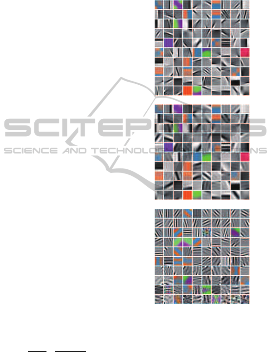
paired basis of the center F. As shown in Figure.2,

each paired basis of the center matches the center of

the corresponding basis of the context, and each of

these three sets has chromatic and achromatic basis.

The joint PDs of a center and its context is

P(C,F) ∝ P(U

)P(U

) =

∏

(21)

Here u

, u

are the k-th elements of U

and U

re-

spectively. The conditional PDs, P(F|C), can be de-

rived using the Bayesian formula as follows:

P(F|C) =

P(F,C)

P(C)

P(U

)P(U

)

P(U

)

∝

∏

(22)

For notational simplicity, we use c

to denote the k-th

context feature u

and f

for the center feature u

Figure 2: ICA basis of the context C and center F. Top: ICs

of the context (columns of A

in (20) ). Middle: Paired ICs

of the center (columns of A

in (20) ). Each IC matches

the center of the corresponding IC in (A). Bottom: Unpaired

ICs of the center (columns of A

in (20)). Each of these

three sets has chromatic and achromatic ICs.

Due to the statistical independence, we only need to

model each element (feature) for contextC and for the

center F from now on. Thus, the terms logP(C) and

logP(F|C) can be calculated as follows:

HierarchicalBayesianModellingofVisualAttention

351

logP(C) =

∑

logP(c

) (23)

logP(F|C) =

∑

logP( f

) (24)

Similarly, P(C|O) and P(F|C,O) can be calculated

from the patches extracted on the target. The single-

scale saliency measure in (17) is derived as follows:

BUTD

= logP(F|C,O) − logP(F|C)

+ logP(C|O) − logP(C)

∑

(logP( f

|O) − logP( f

))

∑

(logP(c

|O) − logP(c

)) (25)

We modeled the probability distribution P( f|O), P(f)

, P(c|O) and P(c) in (25) as generalized Gaussian dis-

tributions (GGD).

4 RESULTS

In this section, we test the models performance of hu-

man gaze prediction in free-viewingand object search

tasks.

4.1 Free Viewing

We used the gaze data in free-viewingstatic color nat-

ural scenes collected by Bruce and Tsotsos (Bruce

and Tsotsos, 2009) to evaluate our model of visual

saliency. This dataset contains human gaze collected

from 20 participants in free-viewing120 color images

of indoor and outdoor natural scenes.

To quantitatively access how well our model

of visual saliency predicts human performance, we

used the receiver operating characteristic (ROC) and

the KullbackCLeibler (KL) divergence measure. To

avoid a central tendency in human gaze (Zhang et al.,

2008), we used the measure described in (Tatler et al.,

2005). Rather than comparing the saliency mea-

sures at attended locations in the current scene to the

saliency measures at unattended locations in the same

scene, we compared the saliency measures at the at-

tended locations to the saliency measures in that scene

at the locations that are attended in different scenes in

the dataset, called shufﬂed ﬁxations.

Our model of visual saliency is a good predictor of

human gaze during the free-viewing of static natural

scenes, outperforming all other models that we tested.

As shown in Table 1, our model has an average KL

divergence of 0.3495 and its average ROC measure is

0.6863. The average KL divergence and ROC mea-

sure for the AIM model in (Bruce and Tsotsos, 2009)

Table 1: ROC metric and KL-divergence for BU saliency of

static natural scenes.

Model KL ROC

(Itti et al., 1998) 0.1130 0.6146

(Gao and Vasconcelos, 2007) 0.1535 0.6395

(Zhang et al., 2008) 0.1723 0.6570

(Bruce and Tsotsos, 2009) 0.2879 0.6799

(Xu et al., 2010) 0.3016 0.6803

0.3495 0.6863

are 0.2879 and 0.6799 respectively, which were cal-

culated using the code provided by the authors.

4.2 Visual Search Tasks

We used the human data described in (Torralba et al.,

2006) for visual search tasks. For completeness, we

give a brief description of their experiment. Twenty-

four Michigan State University undergraduates were

assigned to one of three tasks: counting people,

counting paintings, or counting cups and mugs. In

the cup and painting counting groups, subjects were

shown 36 indoor images (the same for both tasks), and

in the people-counting groups, subjects were shown

36 outdoor images. In each of the tasks, targets were

either present or absent, with up to six instances of

the target appearing in the present condition. Images

were shown until the subject responded with an ob-

ject count or for 10s, whichever came ﬁrst. Images,

subtending 15.8

× 11.9

, were displayed on an NEC

Multisync P750 monitor with a refresh rate of 143

Hz. Eyetracking was performed using a Generation

5.5 SRI Dual Purkinje Image Eyetracker with a sam-

pling rate of 1000 Hz, tracking the right eye.

The training of top-down components of our

model was performed on a subset of the LabelMe

dataset (Russell et al., 2008). We used 198 images

with cups/mugs, 426 images with paintings, and 389

images of street scenes for training. For testing, we

used the stimuli sets shown to human subjects in Tor-

ralba et al’s experiment.

We obtained 447 cups/mugs, 818 paintings, and

1357 people in the labeled training images. For each

target object, we sampled a set of 21x21 patches from

the images. Each set of patches includes patches at

the same location at all the selected scales. For 21x21

patch size, we used only 3 scales. We sampled at

most 3*3 sets of patches for a cup, 5*5 sets for a

painting, and 2*5 sets for a person. We also sampled

the same number of sets of negative patches from the

background in the training images. We obtained the

VISAPP2014-InternationalConferenceonComputerVisionTheoryandApplications

352

PDs, P(C) and P(F|C) , from the negative patches,

and P(C|O) and P(F|C,O) from the object patches.

We obtained the object locations from the cen-

ter of masks in the annotation data, and estimated

P(X|O) for each object category. As discussed in

(Torralba et al., 2006), the horizontal locations of

objects can be modeled by a uniformly distribution.

Therefore, we only used the Gaussian distribution to

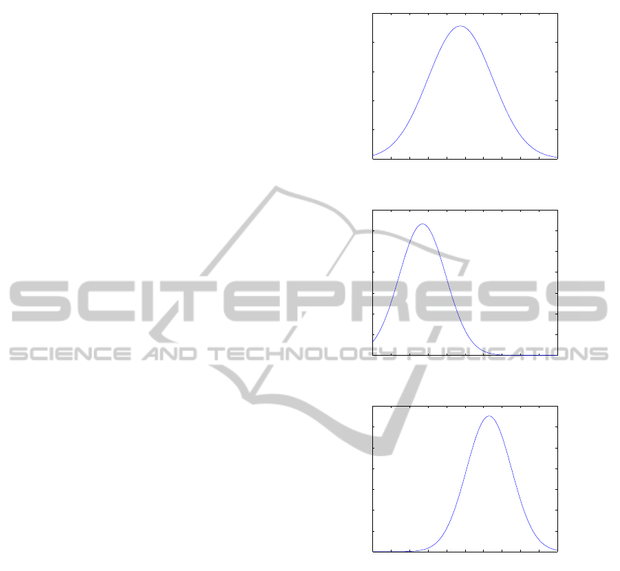
model the vertical locations for each object category.

The PDs of the object locations in the training im-

ages are shown in Fig.3. It was observed that cups are

more likely to be in the middle of the images, paint-

ings appear more frequently on the upper part of the

images, and people on the lower part of the images. It

should be pointed out that we focused on appearance

of targets and contexts and used a simple model for

the object location. In (Torralba et al., 2006), scene

gist was used to model the distribution of object loca-

tions in speciﬁc input image. As discussed in Section

2.3, the location attention in (Torralba et al., 2006)

can also be integrated into our model.

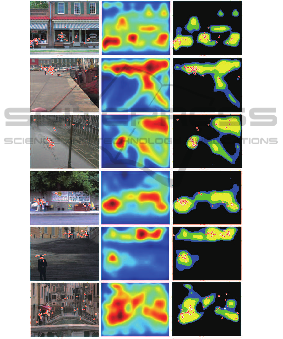
Fig.4 shows several saliency maps and the top

30% most salient regions for the test images used

in the people search task. The saliency maps

were smoothed using a Gaussian kernel with a half-

amplitude spatial width of 1

of visual angle, the same

procedure used in (Kanan et al., 2009; Torralba et al.,

2006) to make comparison with the density maps of

human ﬁxations. The ﬁrst 5 ﬁxations for all 8 sub-

jects were superimposed on the original images (left

column) and the selected regions (right column). As

shown in Fig.4, most of human ﬁxations fell into the

top 10% most salient regions.

In Fig.5, we compared the saliency maps of the

same images for different tasks. The bottom-up

saliency map is same for both tasks. The top-down

effects of the targets on the saliency maps were shown

in the full saliency map and the selected top 30% most

salient regions. As predicted by our model, the paint-

ings became more salient in the painting search task

and the mugs became more salient in the mug search

task.

To examine how well the hierarchical model pro-

posed here predicts human ﬁxations quantitatively,

we adopted the performance measure used in (Tor-

ralba et al., 2006) and (Kanan et al., 2009). The mea-

sure evaluatesthe percentage of each subjects ﬁrst ﬁve

ﬁxations being made to the top 20% most salient re-

gions of the saliency map. The ﬁxation prediction

rates for the three object search tasks were shown in

Table 2. Forcomparison, the results in (Torralba et al.,

2006) were also shown in Table 2, these data were

read from the ﬁgures in their paper. It can be seen

that the BU saliency measure of our model is sim-

0 0.1 0.2 0.3 0.4 0.5 0.6 0.7 0.8 0.9 1

0.5

1.5

2.5

Vertical location, y

p(y) of cups

(a) Cups

0 0.1 0.2 0.3 0.4 0.5 0.6 0.7 0.8 0.9 1

0.5

1.5

2.5

3.5

Vertical location, y

p(y) of paintings

(b) Paintings

0 0.1 0.2 0.3 0.4 0.5 0.6 0.7 0.8 0.9 1

0.5

1.5

2.5

3.5

Vertical location, y

p(y) of people

Figure 3: Distribution of the normalized vertical locations

of objects.(0 means top; 1 means bottom.)

ilar or better than that in (Torralba et al., 2006) for

all three tasks. For the full model, our result is bet-

ter in painting tasks, but not as good as the results

in (Torralba et al., 2006) for mug and people search

tasks. This is because the low-level object features

are used at all scales, the contexts at higher scales are

too coarse and abstract to be discriminative, therefore

for complex objects like pedestrians, the appearance

model is not powerful enough. For small objects like

cups and mugs, the contexts at higher scales are most

from backgrounds, not from objects.

To investigate the effects of patch sizes and scales

on the performance, we re-ran the model using im-

age patches of 11 × 11 pixels at 4 scales. The re-

sults for different patch sizes were similar, with about

HierarchicalBayesianModellingofVisualAttention

353

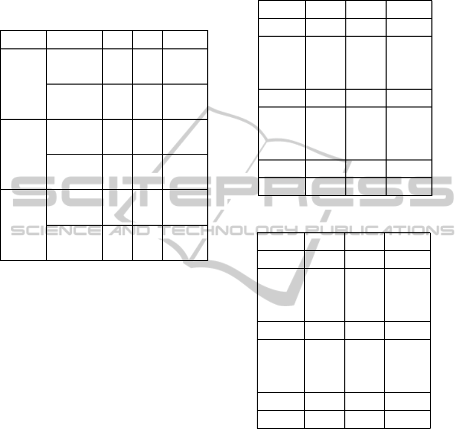
Table 2: Performance comparison in object search tasks. PR

(PresentRate) is for images with target present, AR (Absen-

tRate) for images with target absent. Average is the average

of PR and AR. CGM is the context-guidance model in (Tor-

ralba et al., 2006)

Tasks Models PR AR Average

BU(CGM) 0.42 0.44 0.43

Painting S

0.47 0.43 0.45

CGM 0.57 0.48 0.53

FULL

0.63 0.51 0.57

BU(CGM) 0.71 0.62 0.66

Mug S

0.70 0.61 0.65

CGM 0.82 0.65 0.74

FULL

0.74 0.64 0.69

BU(CGM) 0.63 0.49 0.56

People S

0.67 0.51 0.59

CGM 0.78 0.65 0.72

FULL

0.71 0.58 0.64

2% improvement on the average rate for patch size of

11× 11 at 4 scales.

We also tested the performance of various saliency

measures proposed in Section 2. Due to page limita-

tions, we show the results of 6 selected measures in

Table 3 to Table 5 for the visual search tasks. These

results show several important aspects of the model

proposed here. 1), all saliency measures make bet-

ter predictions than the location measure only. 2), the

bottom-up saliency measures make good predictions

since the targets (e.g., cups, paintings, and people) are

usually salient. 3), the multi-scale saliency measures

are better than single-scale measures. 4), the measure

with TD and BU integrated are better than the bottom-

up only measure.

The results in Table 2 and Table 3 to Table 5 also

show several weaknesses of the current implementa-

tion of our model. First, the Gaussian PD model of

object locations is weak in some cases. For the mug

search task, the location saliency is slightly higher

than the chance level, 20%. Therefore the integration

of the location saliency into the full model does not

make any improvement. This may be because there

were only 447 mugs/cups in the training images. For

the people search task, there were 1357 people in the

training images, and the location measure performs

better (45% average rate). If the object location distri-

bution is estimated by the scene gist, as implemented

in (Torralba et al., 2006), the full model should have

Table 3: Performance of saliency models in predicting hu-

man gaze for the painting search task.

Measure PR AR Average

LOC

0.3644 0.3208 0.3426

SC0

0.4648 0.4267 0.4458

SC1

0.4605 0.4023 0.4314

SC2

0.4032 0.4137 0.4084

0.4663 0.4332 0.4498

BUTD

SC0

0.4577 0.4593 0.4548

BUTD

SC1

0.4548 0.3811 0.4180

BUTD

SC2

0.4075 0.2997 0.3536

BUTD

0.5681 0.4137 0.4909

FULL

0.6298 0.5147 0.5723

Table 4: Performance of saliency models in predicting hu-

man gaze for the mug search task.

Measure PR AR Average

LOC

0.2463 0.2138 0.2300

SC0

0.6634 0.5948 0.6291

SC1

0.6894 0.6138 0.6516

SC2

0.6584 0.5724 0.6154

0.6955 0.6138 0.6547

BUTD

SC0

0.6869 0.5810 0.6340

BUTD

SC1

0.7042 0.6345 0.6693

BUTD

SC2

0.6844 0.5897 0.6370

BUTD

0.7438 0.6448 0.6943

FULL

0.7438 0.6397 0.6917

better performance. Second, the low-level object fea-

tures are not sufﬁciently discriminative with respect

to the backgrounds. As a result, the contribution of

the top-down attention was less than the bottom-up

saliency. In future works, we will include intermedi-

ate and high-level object features and develop more

powerful models of object locations in natural con-

texts.

5 CONCLUSIONS

We made three contributions in this paper. First,

we proposed a biologically inspired, hierarchical

Bayesian model of visual attention. We used multi-

VISAPP2014-InternationalConferenceonComputerVisionTheoryandApplications

354

Table 5: Performance of saliency models in predicting hu-

man gaze for the people search task.

Measure PR AR Average

LOC

0.5512 0.3498 0.4505

SC0

0.6042 0.4778 0.5410

SC1

0.6609 0.4915 0.5762

SC2

0.6732 0.4898 0.5815

0.6708 0.5102 0.5905

BUTD

SC0

0.5536 0.4283 0.4910

BUTD

SC1

0.6449 0.5171 0.5810

BUTD

SC2

0.6967 0.5171 0.6069

BUTD

0.6905 0.5512 0.6209

FULL

0.7127 0.5751 0.6439

scale features and modeled conditional PDs of these

features to measure TD and BU visual saliency. We

optimally combined top-down attention and bottom-

up visual saliency in a Bayesian framework. Second,

we showed that the model can predict human ﬁxations

very well in free viewing and object searching tasks.

Finally, we obtained a range of useful observations on

top-downattention, bottom-up saliency,visual search,

object detection, and the effects of visual context.

These results support the hypothesis that neurons

in the visual cortex may act as estimators of the con-

ditional PDs of visual features in speciﬁc contexts

in natural scenes and the visual features are encoded

progressively downward the hierarchical visual cor-

tex. An ongoing debate in current studies on visual

saliency is whether or not there should be a saliency

map in the brain. In our model, computational units

of the hierarchically organized visual system encode

the conditional PDs of visual variables in natural con-

texts and thus convey saliency information explic-

itly. Therefore, no further complicated operations

are needed to calculate visual saliency and the visual

saliency may distribute at all levels of the visual cor-

tex.

In the pioneering bottom up saliency model (Itti

et al., 1998), multi-scale features were also used, as

in our model. Although both models are biologi-

cally inspired, our model is different from theirs in

the following ways. First, in (Itti et al., 1998), center-

surround differences between a center at a ﬁner scale

and a surround at a coarser scale yield the feature

maps. In our model, the saliency measure was de-

ﬁned based on the conditional probability distribu-

tion of a center in a surround (context). Second, we

used independent components learned from natural

scenes, whereas in (Itti et al., 1998), orientation, color

and intensity features were used. The SUN model

in (Kanan et al., 2009) is most related to our work.

In SUN model, the PD P(O|F) was modeled using

SVM, therefore it is a discriminative approach, dif-

ferent from our generative model, in which P(F|O)

is modeled using GGD. Meanwhile, our model has

multi-scale hierarchical architecture, different from

the single scale in SUN.

ACKNOWLEDGEMENTS

This work is supported by the National Natural Sci-

ence Foundation of China under Project 61175116,

and Shanghai Knowledge Service Platform for Trust-

worthy Internet of Things (No. ZF1213).

REFERENCES

Bell, A. J. and Sejnowski, T. J. (1997). The ”independent

components” of natural scenes are edge ﬁlters. Vision

Res, 37:3327–38.

Borji, A. and Itti, L. (2013). State-of-the-art in visual atten-

tion modeling. IEEE Trans Pattern Anal Mach Intell,

35:185–207.

Bruce, N. D. and Tsotsos, J. K. (2009). Saliency, attention,

and visual search: an information theoretic approach.

J Vision, 9:1–24.

Ehinger, K. A., Hidalgo-Sotelo, B., Torralba, A., and Oliva,

A. (2009). Modeling search for people in 900 scenes:

A combined source model of eye guidance. Visual

Cognition, 17:945–978.

Einhauser, W., Spain, M., and Perona, P. (2008). Objects

predict ﬁxations better than early saliency. J Vis, 8:1–

26.

Elazary, L. and Itti, L. (2010). A bayesian model for

efﬁcient visual search and recognition. Vision Res,

50:1338–52.

Frintrop, S., Rome, E., and Christensen, H. I. (2010). Com-

putational visual attention systems and their cognitive

foundations: A survey. ACM Transactions on Applied

Perception, 7:1–46.

Gao, D., Han, S., and Vasconcelos, N. (2009). Discriminant

saliency, the detection of suspicious coincidences, and

applications to visual recognition. IEEE Trans Pattern

Anal Mach Intell, 31:989–1005.

Gao, D. and Vasconcelos, N. (2007). Bottom-up saliency is

a discriminant process. In ICCV. IEEE.

Gao, D. and Vasconcelos, N. (2009). Decision-theoretic

saliency: computational principles, biological plausi-

bility, and implications for neurophysiology and psy-

chophysics. Neural Comput, 21:239–71.

Gattass, R., Sousa, A. P., and Gross, C. G. (1988). Vi-

suotopic organization and extent of v3 and v4 of the

macaque. Journal of neuroscience, 8:1831–45.

HierarchicalBayesianModellingofVisualAttention

355

Hyvarinen, A. (1999). Fast and robust ﬁxed-point algo-

rithms for independent component analysis. IEEE

Trans Neural Netw, 10:626–34.

Itti, L. and Baldi, P. (2009). Bayesian surprise attracts hu-

man attention. Vision Res, 49:1295–306.

Itti, L., Koch, C., and Niebur, E. (1998). A model of

saliency-based visual attention for rapid scene anal-

ysis. IEEE Trans Pattern Anal Mach Intell, 20:1254–

1259.

Kanan, C., Tong, M. H., Zhang, L., and Cottrell, G. W.

(2009). Sun: Top-down saliency using natural statis-

tics. Visual Cognition, 17:979–1003.

Lee, T. S. and Mumford, D. (2003). Hierarchical bayesian

inference in the visual cortex. Journal of the Optical

Society of America A, Optics, image science, and vi-

sion, 20:1434–48.

Lee, T. S., Yang, C. F., Romero, R. D., and Mumford,

D. (2002). Neural activity in early visual cortex re-

ﬂects behavioral experience and higher-order percep-

tual saliency. Nature neuroscience, 5:589–97.

Navalpakkam, V. and Itti, L. (2005). Modeling the inﬂuence

of task on attention. Vision Res, 45:205–31.

Navalpakkam, V. and Itti, L. (2007). Search goal tunes vi-

sual features optimally. Neuron, 53:605–17.

Olshausen, B. A. and Field, D. J. (1996). Emergence of

simple-cell receptive ﬁeld properties by learning a

sparse code for natural images. Nature, 381:607–9.

Peters, R. J. and Itti, L. (2007). Beyond bottom-up: In-

corporating task-dependent inﬂuences into a compu-

tational model of spatial attention. In CVPR’06. IEEE.

Rao, R. P., Zelinsky, G. J., Hayhoe, M. M., and Ballard,

D. H. (2002). Eye movements in iconic visual search.

Vision Res, 42:1447–63.

Russell, B. C., Torralba, A., Murphy, K. P., and Freeman,

W. T. (2008). Labelme: A database and web-based

tool for image annotation. International Journal of

Computer Vision, 77:157–173.

Serre, T., Oliva, A., and Poggio, T. (2007). A feedforward

architecture accounts for rapid categorization. Proc

Natl Acad Sci U S A, 104:6424–9.

Tanaka, K. (1996). Inferotemporal cortex and object vision.

Annual review of neuroscience, 19:109–39.

Tatler, B. W., Baddeley, R. J., and Gilchrist, I. D. (2005).

Visual correlates of ﬁxation selection: effects of scale

and time. Vision Res, 45:643–59.

Toet, A. (2011). Computational versus psychophysical

bottom-up image saliency: a comparative evaluation

study. IEEE Trans Pattern Anal Mach Intell, 33:2131–

46.

Torralba, A., Oliva, A., Castelhano, M. S., and Henderson,

J. M. (2006). Contextual guidance of eye movements

and attention in real-world scenes: the role of global

features in object search. Psychol Rev, 113:766–86.

Triesch, J., Ballard, D. H., Hayhoe, M. M., and Sullivan,

B. T. (2003). What you see is what you need. J Vis,

3:86–94.

Xu, J., Yang, Z., and Tsien, J. Z. (2010). Emergence

of visual saliency from natural scenes via context-

mediated probability distributions coding. PLoS ONE,

Zelinsky, G. J., Zhang, W., Yu, B., Chen, X., and Samaras,

D. (2006). The role of top-down and bottom-up pro-

cesses in guiding eye movements during visual search.

In NIPS’06. Cambridge, MA: MIT Press.

Zhang, L., Tong, H., Marks, T., Shan, H., and Cottrell,

G. W. (2008). Sun: A bayesian framework for saliency

using natural statistics. J Vis, 8:1–20.

VISAPP2014-InternationalConferenceonComputerVisionTheoryandApplications

356

APPENDIX

Figure 4: Saliency maps and selected regions for the people search task. Each panel shows the original images with the ﬁrst

5 ﬁxations for all 8 participants superimposed (left), the full saliency maps (middle), the top 30% most salient regions of the

saliency maps with the subject ﬁxations (right), where yellow, green, and blue correspond to the top 10, 20, and 30% most

salient regions respectively.

HierarchicalBayesianModellingofVisualAttention

357

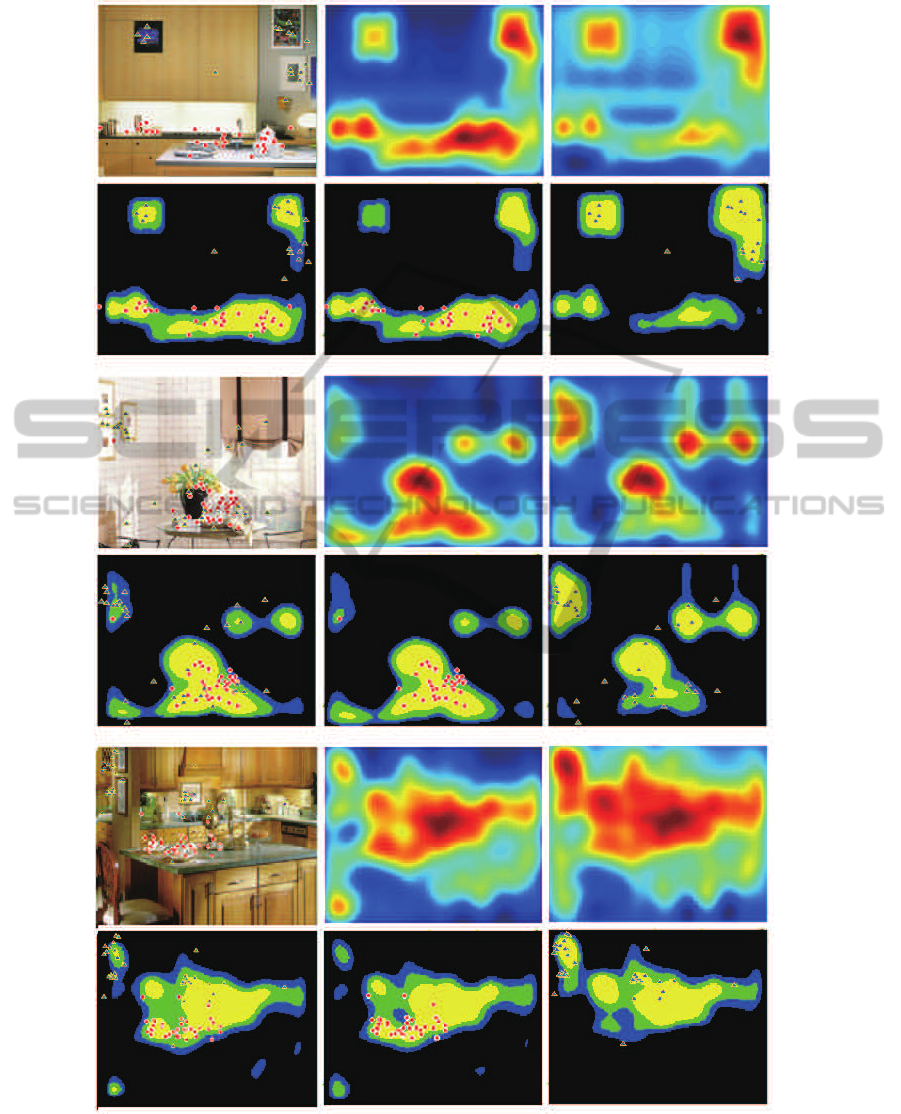
Figure 5: Saliency maps and selected regions for the mug and painting search tasks. The left column of each panel is the

original image (top) and top 30% most salient regions from bottom-up saliency map (bottom) with the ﬁrst 5 ﬁxations for all

subjects superimposed for both search tasks (red circles for mug search and blue triangles for painting search). The middle

column is the full saliency map (top) and its top 30% most salient regions (bottom) for cup search task. The right column is

the full saliency map (top) and its top 30% most salient regions (bottom) for painting search task.

VISAPP2014-InternationalConferenceonComputerVisionTheoryandApplications

358