
Geodesic Mesh Processing with Edge-Front based Data Structures
Hendrik Annuth and Christian-A. Bohn
Computer Graphics & Virtual Reality, Wedel University of Applied Sciences, Feldstr. 143, Wedel, FR Germany
Keywords:
Computational Geometry, Geodesic Distances, Shortest Path, Edge-Front.
Abstract:
In this paper a novel mesh processing data structure is presented which is efficient in runtime and has an
exceptionally low memory consumption. The data structure is extremely versatile and allows investigating
various mesh properties without requiring any pre-processing steps such as triangle subdivision or remeshing.
The data structure uses an edge-front — a sealed path of mesh edges — whose expansion can by altered to
account for individual problem cases. A basic implementation of this data structure — the Minimal Edge Front
(MEF) — has already been successfully used to investigate and resolve inconsistently oriented surface regions
in a surface reconstruction approach based on an iterative refinement strategy.
The MEF is explained in detail and it is augmented to approximate geodesic distances. Our approach allows
us to analyze geodesic surface aspects independent of the mesh triangulation and the processing is limited to
the investigated area. The edge-front enables to deal with open surfaces and to use points as well as lines as a
starting point. The results of the process will be experimentally shown and discussed.
1 INTRODUCTION
Surface Reconstruction by Refinement:
Surface re-
construction creates a 2D subspace in a 3D space that
represents a digital equivalent of a real world physical
surface, which has been scanned with some measur-
ing device. When using the Growing Cell Structures
(GCS) algorithm (Fritzke, 1993) an iterative refine-
ment strategy is applied as a reconstruction process,
such as presented in (Ivrissimtzis et al., 2003). Here, a
current surface estimate of the surface under investi-
gation is constantly optimized by iteratively repeated
operations.
Solving Twisted Surface:
In most computer graph-
ics applications surfaces are oriented in order to use
texturing and efficient rendering techniques. When re-
constructing a surface with GCS the orientation of the
initial surface estimate evolves alongside the surface
in the refinement process.
A current surface estimate in the process is always an
attempt to approximate the entire surface under inves-
tigation. This however means that in early stages some
complex shaped geometry might be represented by a
very crude and simplistic shape. The transition from
that simple to a more sophisticated shape is performed
by a serious of local adaptations. Without any global
overview or supervision, these local adaptations might
produce results that are inconsistent on a global level.
This can lead to surfaces ending up in a local mini-
mum, which can be left when cutting operations are
introduced (Annuth and Bohn, 2010).
It can also lead to inconsistencies in the orientation of
surfaces (see Fig. 1). A mechanism to resolve such
inconsistently oriented surface regions has been pre-
sented in (Annuth and Bohn, 2012). The method ana-
lyzis the mesh connectivity to cut connections in the
mesh to separate ”twisted” surface segments. When
separated, the orientation of such segments could be
swapped independently from each another.
Figure 1: A series of reconstruction stages in the GCS ap-
proach creating an inconsistently oriented surface (top row).
When further optimized, the differently oriented surfaces
remained with a gap in between (bottom left and middle).
The correct reconstruction of the model (bottom right). The
twist occurs, since back and front of the vault have the
same orientation, but the initial GCS estimate is box-shaped,
exposing different orientations for front and back.
To properly integrate into the GCS process, the so-
lution needs to be efficient in runtime and memory
consumption. This necessitates a processing strategy
64
Annuth H. and Bohn C..
Geodesic Mesh Processing with Edge-Front based Data Structures.
DOI: 10.5220/0004718900640075
In Proceedings of the 9th International Conference on Computer Graphics Theory and Applications (GRAPP-2014), pages 64-75
ISBN: 978-989-758-002-4
Copyright
c
2014 SCITEPRESS (Science and Technology Publications, Lda.)

in which only those surface regions are processed,
which are actually involved in a twist and scales to
the problem at hand. The problem of twisted surface
effects the surface on a global level, while an iterative
refinement approach uses a local optimization strategy.
This creates an additional integration problem for a
viable solution. In order to meet these requirement a
novel edge-front based data structure was used — the
MEF. With the MEF the actual resolving method could
be expressed very compactly.
Geodesic Applications:
The MEF can also be applied
to geodesic distance calculations. Making on-surface
distances available for mesh analyzing, searching and
editing processes, has many application cases in ge-
ometry processing. It can be used for mesh param-
eterization to define texture coordinates (Zigelman
et al., 2002). It is also used in mesh segmentation,
where mesh segments are determined, which are then
replaced by B-spline patches to create smooth surfaces
(Krishnamurthy and Levoy, 1996). When comparing
the distribution of distances the process can be used
for topology matching (Hilaga et al., 2001). In ani-
mation a mesh decomposition is needed to distinguish
surface components in the animation of a model, which
again can be determined by analysing on-surface dis-
tance distribution (Katz and Tal, 2003). When using
procedural textures on complex meshes geodesic co-
ordinates can be used to determine a transfer function
between the space of the procedural function and the
topological space of the mesh (Oliveira et al., 2010).
All these applications require a surface distance met-
ric which can be established with geodesic distances.
Geodesic distance calculations can be divided into ex-
act and approximated solutions.
A first implemented exact solution (Kaneva and
O’Rourke, 2000) used a graph based search strategy
on a sequence tree and was theoretically suggested in
(Chen and Han, 1990). The algorithm has quadratic
time complexity. In most currently used applications
approximated solutions are used. The fast marching
method (FMM) (Sethian, 1995) was introduced to find
approximate distance solutions for triangular meshes
(Kimmel and Sethian, 1998). In the approach, dis-
tances are calculated from a starting vertex. All ver-
tices currently reachable are considered and the closest
is added to the ”known” vertices. When a vertex is
newly added, all new vertices reachable from this new
vertex are added to the ”reachable” vertices. By al-
ways adding the closest vertex, the FMM works like
the algorithm of Dijkstra. Even so significantly more
precise approximation methods exist, which are only
marginally slower than FMM, due its simple imple-
mentation FMM approaches are the most widely used.
The accuracy of the approach strongly depends on
the given triangulation, since the discrete calculation
points are determined by the vertex distribution.
To be more independent of the given mesh triangula-
tion and to increase accuracy many subdivision tech-
niques, adding more edges into the initial mesh, where
introduced (Lanthier et al., 1997). In (Kanai and
Suzuki, 2000) the shortest path is first calculated on the
original edges of the mesh with Dijkstra’s algorithm
and then the area of the resulting path is repeatedly sub-
divided to repeat the search, until a certain subdivision
level is reached.
In (Mitchell et al., 1987) an exact solution was pre-
sented. Here, the mesh was subdivided in so called
windows to guarantee the possibility to compute an ex-
act shortest path on the given mesh edges. When estab-
lished, the path can again be calculated with Dijkstra’s
algorithm. The suggested method has a worst case
runtime complexity slightly above quadratic. How-
ever, when first implemented (Surazhsky et al., 2005)
it proved to be significantly more efficient in prac-
tice. Due to the intensive subdividing of the windows,
the approach has a significantly higher memory con-
sumption than other approaches. Based on the initial
approach an approximate solution was presented in the
same work, which reduced this problem. The approach
was extended to additionally allow line segments as
starting point in (Bommes and Kobbelt, 2007). A more
detailed overview on the subject of geodesic path cal-
culation can be found in (Bose et al., 2011).
A recent breakthrough in shortest path calculation has
been achieved (Crane et al., 2012), which has a close
to linear runtime. Here, the problem is solved by
transferring it into a Poisson equation.
In the following we present an approximate geodesic
distance calculation with a memory consumption lin-
early related to the length of the investigated distance.
At the same time, the process is efficient in runtime,
requires no additional subdividing of the mesh and
its processing strategy can easily been altered to ac-
count for individual problem cases (see section 2.3).
First, the data structure which led to this approach is
introduced. This section focuses on the calculation of
edge-wise distances on a given mesh (see section 2.2).
2 APPROACH
Surface twists are a global phenomenon, while the
refinement operations of the GCS approach optimize
on a local level. The twist solving mechanism pre-
sented in (Annuth and Bohn, 2012), however, needed
to properly integrate into the iterative refinement pro-
cess achieved by the chosen semi-local processing
strategy.
GeodesicMeshProcessingwithEdge-FrontbasedDataStructures
65

It involves surface computations at a limited domain
around a point of interest and having control over the
expansion of the processed area. Additionally the
processing should create a small memory footprint
enabling the processing of vast surface areas.
In the following, first, the Vertex Front (VF) a pre-form
of the MEF data structure is presented. Then a defi-
nition followed by a detailed explanation of the MEF
data structure is given. The Minimal Distance Front
(MDF) is presented enhancing the processing strategy
to include on-surface distances. Last, based on these
data structures, an efficient way of calculating minimal
connecting paths between vertices is presented.
2.1 Vertex Front
The inspiration for the VF came from accessing vertex
neighborhoods. First degree neighbors can easily be
accessed by iterating through all connected edges of
a vertex. When however the first neighborhood of an
edge, a triangle, or when higher degrees of neighbor-
hoods are accessed, an advanced concept is needed.
Algorithm 1: Vertex Front.
1: Clean all containers: V
f ront
= V
old
= V
new
= {}
2: Add starting point vertex/vertices to V
f ront
3: while Expansion level not reached AND
front not empty: n
exp
> 0 ∧ |V
f ront
| > 0 do
4: repeat
5: Pick not processed vertex v
x
from V
f ront
6: Get first degree neighborhood N
x
of v
x
7: repeat
8: Pick not processed vertex v
y
from N
x
9: if v
y
is a new vertex:
v
y
/∈ V
old
∧ v
y
/∈ V
f ront
∧ v
y
/∈ V
new
then
10: Add v
y
to new vertices: V
new
= V
new
∩ v
y
11: end if
12: until All vertices in N
x
have been processed
13: until All vertices in V
f ront
have been processed
14: Swap containers:
V
old
= V
f ront
∧ V
f ront
= V
new
∧ V
new
= {}
15: Decrement expansions: ∆n
exp
= −1
16: end while
The Vertex Front (VF) is an expandable set of vertices
(see algo. 1). It is initialized with a set of vertices (see
line 2 in algo. 1), e.g., the vertices of a triangle. These
initial vertices can then be expanded. The VF includes
three data containers for old
V
old
, current
V
f ront
and
new
V
new
vertices. These containers need to offer
optimized operations to add, to find, and to iterate
through vertices. In the presented implementation
a
red
-
black
tree is used. When the current front is
expanded the algorithm iterates through all vertices
in
V
f ront
(see line 13 in algo. 1). The surrounding
vertices
N
x
of each vertex
v
x
in
V
f ront
are tested, for
being either vertices of the previous front
V
old
(empty
on initial expansion) or of the current front
V
f ront
or
if they are actually new and have not yet been added
to
V
new
. After processing all vertices, the containers
are swapped (see line 14 in algo. 1). The old front
is replaced with the current one, the current front is
replaced with the new vertices, and the new vertex
container is cleaned for the next expansion. After the
expansion,
V
f ront
contains all un-processed vertices
reachable from the former front.
The VF is an efficient way to investigate the surround-
ings of a vertex. It is easy to implement and works on
a semi-local level. It does not take advantage of the
2D characteristics of a surface to make the expansion
process more runtime efficient. Its most important dis-
advantage is the front
V
f ront
being defined as a loose
set of unconnected vertices. These vertices, depend-
ing on the underlying mesh, are often scattered and
do not expose a consistent ordered front line, as an
edge-fornt does (see below). This vertex based front
does not separate the surface in two clearly distinct
surface areas. A front expansion direction cannot be
defined for the VF. So directing the expansion to in-
vestigate, for instance, the inside of a circle of vertices
is not possible. When a front collides with itself, it is
indeterminable for the process. Neighboring vertices
in the front cannot be distinguished from those coming
from far distant segments of the front.
2.2 Minimal Edge Front
A MEF consists of one or multiple closed edge paths
of mesh edges that enclose all vertices of a certain
edge-wise distance to an initial starting point. This
starting point can be one or several vertices or a closed
not self-intersecting edge path, for instance, the out-
line of a triangle. The edge paths have a front side
where the expansion takes place and a back side where
the already processed surface connects. In that sense,
the MEF behaves like a sweep line algorithm where
calculations only take place at the front of the current
sweeping line. In contrast to most such techniques,
the MEF creates no additional geometric support struc-
tures of any kind, but only uses the given mesh edges.
Edge paths are allowed to have common edges and
vertices, but only if both paths touch with their back
sides, touching or crossing front sides are invalid.
For example, if a MEF is expanded two times from
a single vertex as starting point, it will enclose all
vertices which are connected to the initial vertex by
two mesh edges (see (a) in Fig. 2).
A MEF is ’minimal’ in the way that the vertices it
surrounds cannot be enclosed by a smaller number of
GRAPP2014-InternationalConferenceonComputerGraphicsTheoryandApplications
66
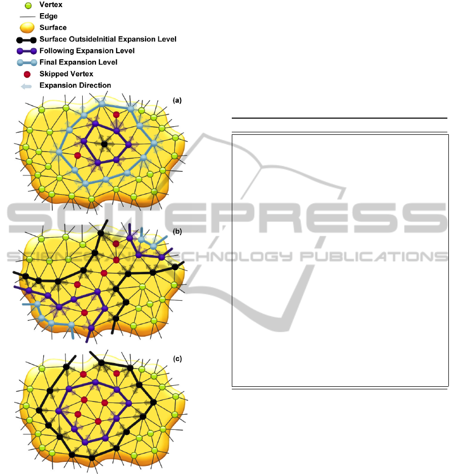
Figure 2: Different cases while expanding a Minimal Edge
Front: (a) expansion from an initial vertex to the second
expansion level; (b) collision and merging while expanding
an edge front; (c) Annihilation of an edge-front that can not
be expanded any further.
mesh edges, unless a front collision would have to be
executed earlier to decrease the number of edges (see
below on collision).
Implementation:
While the VF has a loose set of un-
connected vertices
V
f ront
as a front, the front of the
MEF is defined by closed edge paths, represented as
doubly linked lists (see algo. 2). So for every list ele-
ment
e
x
of such an edge path previous and posterior
edges can be investigated. The process includes differ-
ent containers. In
E
f ront
are the edge elements of the
current front for a completed expansion level.
E
new
contains the new edge elements of a front in progress.
V
f ront
contains the vertices of the current front, needed
to detect collisions. In contrast to the VF,
V
f ront
can
include duplicates, since edge paths can run to one ver-
tex twice. Again these containers can be implemented
as red-black trees.
Algorithm 2: Minimal Edge Front.
1: Clean all containers: V
f ront
= E
f ront
= E
new
= {}
2: Add starting vertex or edge path to V
f ront
and E
f ront
3: if Starting point is vertex: E
f ront
= {} then
4: Translate vertex into edge path
5: end if
6: while Expansion level not reached AND
front not empty: n
exp
> 0 ∧ |V
f ront
| > 0 do
7: repeat
8: Take an edge path element e
x
out of E
f ront
9: Calculate the edge path segment E
x
10: Minimize edge path segment E
x
11: repeat
12: Add vertices from E
x
to front V
f ront
13: if Vertex was already in V
f ront
then
14: Split path E
x
at collision
15:
Minimize the edge path segments in
E
x
16: end if
17: until All vertices of E
x
have been added
18: Connect segment(s) E
x
to the edge front
19: Delete processed elements from containers
20: until No more elements to process: E
f ront
= {}
21: Swap containers: E
f ront
= E
new
∧ E
new
= {}
22: Decrease expansions: ∆n
exp
= −1
23: end while
Expansion:
When the edge-front defines a complete
extension level, all edge path elements are in
E
f ront
and
E
new
is empty. When this front is expanded all
single edge elements in
E
f ront
need to be expanded,
creating a new edge path added to
E
new
. When all
former edges of a previous expansion level are ex-
panded and
E
f ront
is empty (see line 20 in algo. 2),
a new expansion level is reached (see (a) in Fig. 2).
Then the content of
E
new
and
E
f ront
is swapped (see
line 21 in algo. 2), so
E
new
is empty again and
E
f ront
contains the new expansion level. The parameter
n
exp
determines the number of expansion levels performed
to reach the desired final front state.
Single Edge Expansion:
The expansion of the front
to a new expansion level includes the expansion of
single edge path element, as illustrated in Fig. 3. The
expansion of a single edge path element starts by pick-
ing one edge path element of the former front from
E
f ront
(see line 8 in algo. 2). Since edge path ele-
ments are doubly linked list elements, the edge path
GeodesicMeshProcessingwithEdge-FrontbasedDataStructures
67
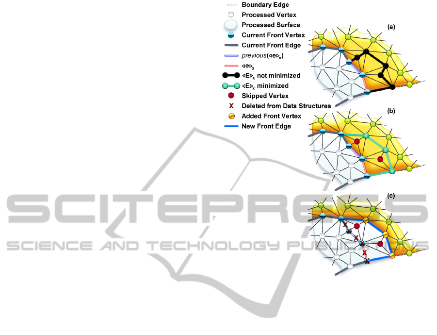
element previous to the picked one can be accessed.
Now the process has two edges with a vertex in be-
tween. The process iterates through all vertices, which
are connected to that vertex in between and that lie in
expansion direction. The path of edges
E
x
connect-
ing those vertices is determined (see (a) in Fig. 3 and
line 9 in algo. 2).
E
x
is supposed to be added to the
front. First, however, the path needs to be minimized
(see (b) in Fig. 3 and line 10 in algo. 2). Whenever the
edge path runs through two edges of a triangle — the
third not being part of the path — the edge path can
be shortened by redirecting the path through that third
edge (see (b) in Fig. 3). Given no collision takes place,
the shortened path
E
x
can be connected with the
edge-front and its edge path elements added to
E
new
(see (c) in Fig. 3 and line 18 in algo. 2). Vertices and
edge path elements which after the expansion lie be-
hind the current front and are now part of the processed
surface can be deleted from the fronts data structures
(see line 19 in algo. 2).
Since MEF bases on edges, a vertex as a starting point
represents an anomaly. However, when using one of its
triangles as an edge path adding one edge incident to
the vertex into
E
f ront
— so it is expanded for the next
expansion level — and the other two into
E
new
— so
they will not be expanded for the next expansion level
— the next expansion builds the front in one edge-wise
distance to that vertex (see (a) in Fig. 2).
Annihilation:
When the minimization of
E
x
leaves
no remaining surface area, the front has been annihi-
lated and ceases to exist (see (c) in Fig. 2). Annihila-
tion of an edge-front often marks the end of a search
process, since the front cannot be further expanded.
Boundaries:
When an edge-front is expanded at a
boundary its vertices are deleted from
V
f ront
, since
collisions cannot take place anymore. Its edge ele-
ments are deleted from the
E
f ront
, since they cannot
be expanded anymore. However, the edge path ele-
ments are kept in the list. From a memory efficiency
perspective this is not ideal, since all boundary edges
passed by the MEF are kept using up memory. How-
ever this implementation has the advantage that edge
paths are always closed and complete, making special
case handling unnecessary.
Collision:
Since an edge-front defines a continu-
ous contour, instead of an unorganized vertex set,
collisions can be detected, and have to be detected,
to inhibit fronts from permeating one another (see
(b) in Fig. 2).
The detection of collisions takes place at a single edge
expansion (see Fig. 4). When a former edge path
element has been expanded and minimized, a new
expansion path segment
E
x
can be added to the
front. Before a new path is connected, it needs to be
Figure 3: Expansion of single edge path element: (a)
the new edge path segment
E
x
in front of
e
x
and
previous(e
x
)
is determined; (b) the segment is minimized
in length; (c) the new segment is connected to the front and
passed front elements are deleted from their corresponding
data structures. Note that more than the initial two edge path
elements have been deleted.
tested if it collides with an existing edge-front. All
vertices of the new path are successively added to the
front vertices
V
f ront
(see line 12 in algo. 2). When a
vertex had already been added to
V
f ront
, a collision
took place (see (b) in Fig. 4). The path in
E
x
is
split (see line 14 in algo. 2) and the new path segments
need to be minimized again (see (c) in Fig. 4 and
line 15 in algo. 2). The collision test needs to be vertex
based, since a collision can involve one vertex only
(see (b) in Fig. 4). A single edge element expansion
can include several collisions (see Fig. 4). When all
collision tests are performed, the possibly separated
segments in E
x
are connected to the front.
Minimum Pathways:
Pathways with a perimeter of
only three vertices (see Fig. 5) need consideration in
the implementation of the MEF.
When a new expansion path segment
E
x
has been
calculated and minimized it is connected to the pre-
existent edge-front. When minimum pathways exist in
a mesh, it is possible for that pre-existent edge-front to
be entirely skipped by the minimization process, while
E
x
contains a valid new edge-front purely by itself.
GRAPP2014-InternationalConferenceonComputerGraphicsTheoryandApplications
68

Figure 4: Several collision cases at a single edge path ele-
ment expansion: (a) determination of path segment
E
x
;
(b) the path segment is minimized and five collisions are
detected; (c) the collisions split the path into six which are
again minimized and two of them are annihilated; (d) finally
four new path segments are connected to the front.
Figure 5: Neck and Back of the Dragon model are connected
by a minimum pathway of three vertices perimeter.
This creates a variety of very implementation specific
special cases when a front at a minimum pathway is
expanded or collides. However, when considered, they
are easily solvable.
2.3 Minimal Distance Front
The presented MEF is an efficient processing tool to
analyze and search aspects concerning the connectivity
in a mesh. From a connectivity focused perspective
any vertex connection or edge is equally valued. This
setting therefore only considers discrete mesh connec-
tivity aspects in its calculation. If, for instance, vertex
positions are altered and thereby the mesh geometry,
the MEF processing would remain unchanged. The
MEF however exposes a front line straightened by the
path minimization. This front line can be directionally
set in relation to the surface, establishing on-surface
distances to the front line. The Minimal Distance
Front (MDF) (see algo. 3) is a MEF with a distance led
selection process for the expanded edge path elements.
Algorithm 3: Minimal Distance Front.
The following algorithm is the result of a modified MEF algo. 2
Color code: Newly added and removed algorithm aspects.
1: Clean all containers: V
f ront
= E
f ront
= E
new
= {}
2: Add starting vertex or edge path to V
f ront
and E
f ront
3: if Starting point is vertex: E
f ront
= {} then
4: Translate vertex into edge path
5: end if
6: Add antisipated distances to D
exp
7: while Expansions not empty AND
next one does not exceed maximum distance:
|D
exp
| > 0 ∧ min(D
exp
) <= d
max
Expansion level not reached AND
front not empty: n
exp
> 0 ∧ |V
f ront
| > 0 do
8: Pick smallest distance element e
x
from D
exp
repeat
9: Take an edge path element e
x
out of E
f ront
10: Calculate the edge path segment E
x
11: Minimize edge path segment E
x
12: repeat
13: Add vertices from E
x
to front V
f ront
with on-surface distance d
start
and direction d
start
14: if Vertex was already in V
f ront
then
15: Split path E
x
at collision
16: Minimize the edge path segments in E
x
17: end if
18: until All vertices of E
x
have been added
19: Connect segment(s) E
x
to the edge front
20: Delete processed elements from containers
21:
Add antisipated distances of new elements to
D
exp
22: Add all edge path elements to current front:
E
f ront
= E
f ront
∩ E
new
∧ E
new
= {}
until No more elements to process: E
f ront
= {}
Swap containers: E
f ront
= E
new
∧ E
new
= {}
Count down expansions: ∆n
exp
= −1
23: end while
To select an edge path element for expansion depen-
dent of the resulting distance to the starting point
makes the anticipation of these distances necessary.
All these anticipated distances with their associated
GeodesicMeshProcessingwithEdge-FrontbasedDataStructures
69
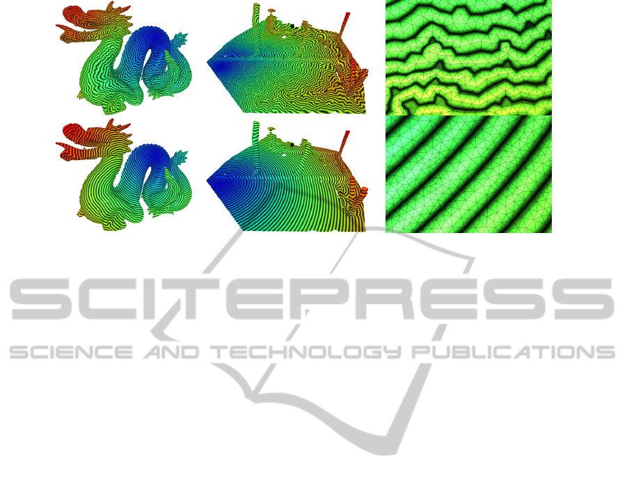
Figure 6: Comparison of MEF and MDF: Distance field on the Dragon (left column), the Heating Pipes (middle column) and a
distance field close up (right column). The distances in the MEF (top row) represent discrete edge counts, while the MDF
(bottom row) represents geometric distances. Due to skipped vertices and discrete distances in case of the MEF, all vertices of a
triangle can have the same distance, creating a unicolored triangle.
edge path elements are added into a container, which
orders them by their anticipated distances. Again, a
red
-
black
tree is suitable for this task. The MEF has
discrete expansion levels, defined as all expansions
needed to move the front one single edge forward (see
line 20 in algo. 2). The MDF is not bound to such
distinct levels as difined by
n
exp
, instead a front de-
fines the farthest distant edge path to a starting point
not exceeding a certain on-surface maximum distance
d
max
(see line 7 in algo. 3). In Fig. 6 the difference of
these expansion behaviors is illustrated.
When front vertices are added to
V
f ront
additionally
their on-surface distance
d
start
and the on-surface di-
rection toward the starting point
d
start
are added (see
line 13 in algo. 3). For the initial vertices
d
start
is zero.
For a single vertex
d
start
is set to the zero vector. For
a vertex of an edge path being the starting point (line)
d
start
can be calculated similar to a boundary normal
of a vertex at a mesh boundary, perceiving the backside
of the edge path (opposite side to the front expansion
direction) as a surface boundary.
Expansion:
The MDF continuously expands with the
expansion of every single edge path element, in con-
trast to the MEF, where all former edge path elements
are expanded to reach the next discrete expansion level.
When a single edge path element in the MDF is ex-
panded, the element with the smallest anticipated on-
surface distance is selected (see line 8 in algo. 3). The
smallest distance is chosen to keep the front at mini-
mum distance to the starting point. The element ex-
pansion itself remains unchanged to the MEF.
When an edge path element
e
x
has been expanded,
the vertices of the new edge path segment
E
x
are
added to
V
f ront
(see line 13 in algo. 3). For every given
vertex
v
x
of the new edge path additionally distance
d
start
and vector d
start
need to be calculated.
The previous edge-front is perceived as a collection of
separated spatial subdivisions delimited by planes in
between them. Those subdivisions are either associ-
ated with an edge, or in between two edge subdivisions,
with a vertex.
A subdivision of an edge
e
sub
in between vertex
v
le f t
at its left and
v
right
at its right, is a space determined
by two planes one intersecting
v
le f t
and the other one
intersecting v
right
(see (b) in Fig. 7).
For a vertex
v
x
to be considered inside a subdivision,
it has to lie on or above both of these planes (see
(a) in Fig. 7). Both planes run parallel to the normal of
triangle
t
sub
lying on the backside of
e
sub
and parallel
to
d
start
of either
v
le f t
for the left plane and
v
right
for
the right plane (see (b) in Fig. 7).
The calculation starts by identifying the subdivision
which covers the vertex
v
x
under investigation. First
the subdivision associated with the edge of
e
x
is
tested.
v
x
might be inside of this subdivision, right,
or left from it. If
v
x
lies left from it, the previous sub-
division of the front
previous( e
x
)
is tested, if
v
x
is
right from it the next subdivision is tested
next(e
x
)
.
When
v
x
lies first at the left and then at the right of
the following subdivision or vice versa,
v
x
lies in the
subdivision of the vertex in between. It is sensible to
limit the number of tested subdivisions. In the pre-
sented implementation not more than
5
subdivisions
are tested. If this limit is exceeded the result of the
search is set to the subdivision associated with the ver-
tex in between
e
x
and
previous( e
x
)
as a fallback
solution. This fallback is also used in case a subdivi-
sion can not be calculated, since t
sub
does not exist or
an accessed vector d
start
is the zero vector.
For
v
x
lying in the subdivision of a vertex
v
sub
the cal-
GRAPP2014-InternationalConferenceonComputerGraphicsTheoryandApplications
70

Figure 7: Calculation of
d
start
and
d
start
: (a) with all aspects
combined; (b) the subdivision of edge
e
sub
; (c) 1. the deter-
mined distance of
v
x
to the subdivision planes; 2. which is
used to scale
d
start
of
v
le f t
and
v
right
; 3. finally the normal-
ized average of these vectors is calculated as a first estimate
of
d
start
for
v
x
; (d) this first estimated vector is projected
onto the surface to determine the intersection point
p
connect
of
e
sub
with the starting point path of
v
x
. Note the subdivi-
sion planes do not necessarily intersect at the starting point.
culations are simple.
d
start
for
v
x
is the distance form
v
x
to
v
sub
plus the distance back to starting point
d
start
form
v
sub
, which already has been calculated and can
be accessed through
V
f ront
.
d
start
is the normalized
vector from v
x
to v
sub
.
When
v
x
lies in the subdivision of an edge
e
sub
, a first
estimate of
d
start
is approximated (see (c) in Fig. 7).
The direction of
d
start
for
v
x
needs to lie in between
d
start
of
v
le f t
and
d
start
of
v
right
. To what degree one of
these vectors is represented in
d
start
should resemble to
which plane
v
x
lies closer. Since a low distance implies
more importance, the relation from representation to
distance is inversely proportional. So,
d
start
of
v
le f t
is scaled to the distance of
v
x
to the right plane and
d
start
of
v
right
is scaled to the distance of
v
x
to the left
plane. Then the normalized average of these vectors
is used as a first estimate for
d
start
for
v
x
. Now,
d
start
represents the direction to the starting point, assuming
the surface progresses like a plane.
When curved, this first estimate needs to be projected
onto the surface (see (d) in Fig. 7). This is achieved
by setting-up another plane which has
v
x
as its ori-
gin point and runs parallel to the estimated vector for
d
start
and again to the normal of triangle
t
sub
. The
point
p
connect
, where this plane intersects with
e
sub
,
represents the point where the on-surface path from
the starting point to
v
x
crosses the front. With this
intersection point distance
d
start
and vector
d
start
can
be determined for v
x
.
d
start
of
v
x
is the distance from
v
x
to
p
connect
plus the
distance back to the starting point. The latter dis-
tance is again calculated as the average of
d
start
of
v
le f t
and
v
right
inversely proportionally weighted by
the distances to the subdivision planes. The final
d
start
for v
x
is the normalized vector from v
x
to p
connect
.
When a single edge expansion has been finished and
the segment(s) in
E
x
have been connected to the
front (see line 19 in algo. 3), the process iterates
through all new front edges. The on-surface distances,
their expansions would lead to, are anticipated. Then
edge path elements with these anticipated distances
are added to D
exp
(see line 21 in algo. 3).
This anticipated distance for an edge path element
e
x
is calculated as the maximum distance
d
start
,
which would be created. So the
d
start
values of all
vertices in the edge path segment
E
x
, that would be
created, have to be determined.
d
start
can be calculated
as it has been calculated before, when adding new
vertices to the front.
2.4 Calculating Connection Path
One out of many applications of the presented data
structures is calculating a connection path between
two vertices in a mesh. To accomplish that, two fronts
are alternatingly expanded from one vertex and new
front vertices are tested for overlapping both fronts.
When one front cannot be further expanded the vertices
are not connected, otherwise an overlapping vertex is
found lying in the middle of the path between the initial
search vertices. With the new vertex the process can
be recursively repeated until vertices are adjacent to
each other, and their edges are added to the connection
path. When all recursive search processes for vertices
have been brought down to adjacent vertices, the entire
path has been determined.
In order to search for the edge-wise shortest connection
path the VF as well as the MEF can be applied (see
Fig. 8). The MEF is more efficient in runtime and
memory consumption. Since every edge is equally
valued an edge-wise shortest connection path is usually
one of many possible paths of the same edge-wise
length.
The MDF determines the shortest on-surface path (see
Fig. 8). Its length can be calculated as the sum of
the distances
d
start
to the first overlapping vertex of
both initially started fronts. The length resembles the
one of the path actually projected onto the surface,
i.e., a path that can run across a triangle. However,
the calculated path is constructed from existing mesh
GeodesicMeshProcessingwithEdge-FrontbasedDataStructures
71
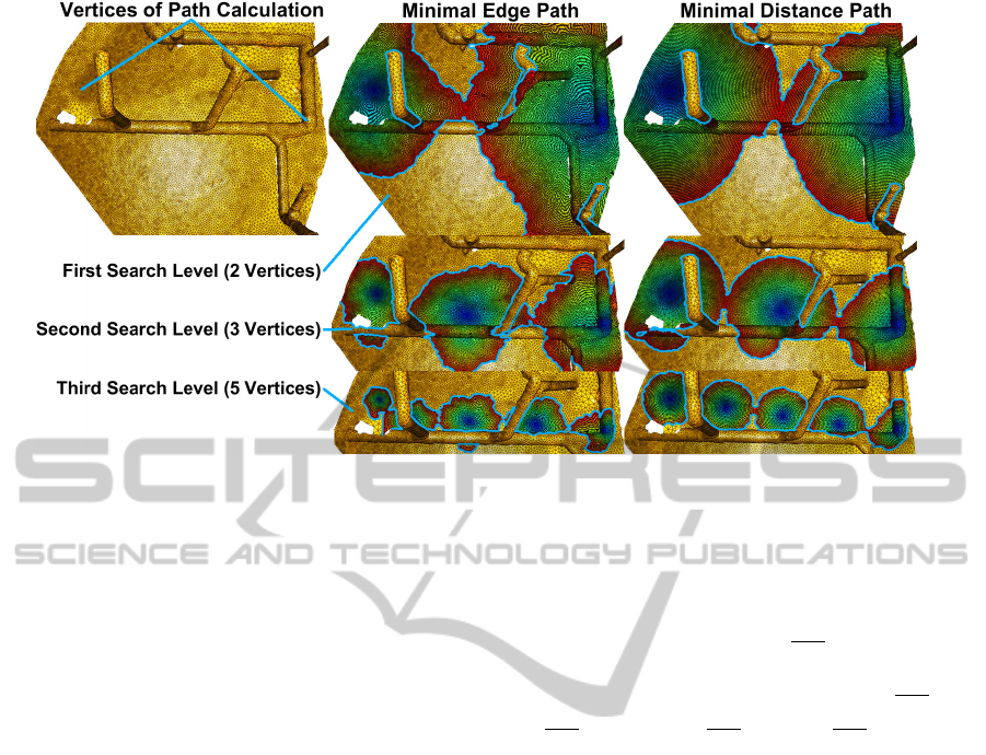
Figure 8: Calculation of a connection path between two vertices (top left) with the MEF (middle column) and the MDF (right
column). Showing the first (top), the second (middle) and the third (bottom) recursive search level. Note how the expansion of
the MEF is determined by the local triangle resolution and the equal edge-wise expansions differ in size and shape.
edges and does not resemble the projected path. This
projected path would be a valuable additional asset in
geometry processing, since it is independent from the
given mesh edges, and could potentially be calculated
with the
d
start
vectors. Note that the MDF based path
calculation is only an example of applying the pre-
sented data structure, which could easily be optimized
as discussed in the conclusions. However, this would
not have served the introduction of the presented edge-
front based data structures.
3 RESULTS
Theoretical Analysis of Complexity:
All upcoming
complexity discussions concerning VF, MEF and MDF
are considered to be performed on a flat infinite regular
grid, where every vertex is connected to exactly six
neighbors and all edges in the grid are of the same
length. The benefit of this assumption is that the VF,
MEF and MDF expand almost the same way — circu-
lar. The number of processed surface elements (area
of a circle) and the length of the front (circumference)
are then easy to calculate. Also cases such as front an-
nihilations, collisions and fronts reaching boundaries
do not need consideration.
Shortest Path Calculation:
The calculation of the
shortest connecting path nicely demonstrates the ad-
vantages of the presented semi-local processing prin-
cipal. When the vertices under investigation are not
connected, only the smaller surface segment is fully
processed and the calculation is thereby held as local
as possible. When determining a connection path of
a length
d
path
the maximum memory consumption is
the one of the two initial circular fronts which radiuses
are half of the path length,
2 · (2π
d
path
2
)
. Here, the pro-
cessed area is the area of the initial two circular areas,
plus the ones of the recursive descent,
2 · π(
d
path
2
)
2
+
4 · π(
d
path
4
)
2
+... + n · π(
d
path
n
)
2
= 1 ·π(
d
path
1
)
2
. The cal-
culation effort only depends on the length of the path
and is independent of the mesh size. With a memory
consumption proportional to the square root of the
processed surface area the operation has a very small
memory footprint. The runtime complexity of all the
fronts is
O(n log n)
, while
n
is the number of processed
mesh elements. All
n
elements are processed and ac-
cessed for a constant number of times and balanced
trees are used for all element accesses O(log n).
Since the same surface is processed multiple times, the
presented shortest path calculation has a bigger con-
stant
c
in runtime than the Dijkstra based shortest path
calculation algorithms mentioned in the introduction.
However, this advantage is achieved by storing all vis-
ited vertices. Therefore, their memory consumption
is proportional to the processed surface area, instead
of its square root. Additionally the presented path cal-
culation could by optimized by taking advantage of
the search direction as in the
A∗
algorithm. Also the
already calculated fronts of previous recursive search
levels could be used to narrow the search domain.
Minimal Edge Front:
The presented MEF is a very
fast way for gaining edge-wise distances and other
mesh connectivity related information. On average for
1000
different starting vertices, a MEF needs
0.343s
to
GRAPP2014-InternationalConferenceonComputerGraphicsTheoryandApplications
72
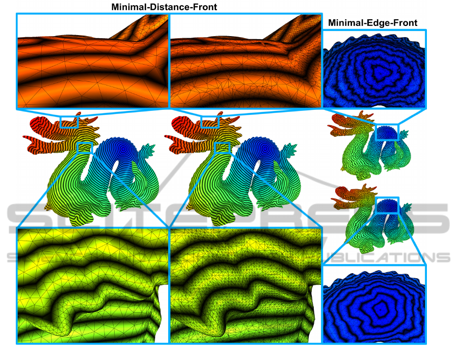
Figure 9: Illustration of a distance field on a reconstruction (# triangles:100K) of the Dragon model (first column) and the
original (# triangles: 871K) Dragon model (second column). Even so the dragons expose very different triangle distributions
and shapes, the local distance lines progress similar on both models. The same demonstration for the MEF (third column)
exposes very different progressing fronts for the reconstructed (bottom) and original (top) model already at the starting point.
visit all
438K
vertices of the Stanford Dragon model,
while the maximum edge count is
3069
. The same
test performed with the VF needs
0.531s
on average.
The MEF exploits the properties of a 2D surface for
its efficiency by using a minimized directed front line
representing a 1D contour. Only elements ahead of
the front are processed and the front is minimized and
thereby many elements are skipped in the process.
Additionally the connected and sealed edge-front is
a more meaningful representation of the surface area
under investigation. It can detect and localize colli-
sions and due to the straightened front line additional
surface aspects can be set in relation to the front.
Minimal Distance Front:
Geodesic distance calcu-
lations with an edge-front can be performed with the
MDF. Using on-surface distances makes the MDF ex-
pansion more independent of the given mesh triangula-
tion and it performs equally well even on challenging
triangulations, as illustrated in Fig. 9.
When a vertex cannot be attributed to a subdivision
in the MDF distance calculation, the fallback solution
uses the distance to the vertex where the initial ex-
pansion took place. This distance estimate is likely
to overshoot the actual front-to-vertex distance. Since
minimum distance expansions are selected, these pos-
sibly oversized estimates are less likely to be selected.
This gives the distance approximation process a certain
self-correction property making it more robust.
When the MDF is performed
1000
times on the Dragon
model it takes
1.420s
on average and uses only
2334
edges at its maximum. The latter confirms a more
straightened circular front, since fewer edges are re-
quired. The MDF is less efficient than the MEF, since
it additionally involves the distance calculation. Also
the MDF with its anticipated distances always needs
to be one step ahead of the current front. Also, the
distances anticipation has to be performed on all ex-
pandable edges, such that many of them are likely to
be skipped and never to be expanded.
However, the presented implementation has been built
GeodesicMeshProcessingwithEdge-FrontbasedDataStructures
73
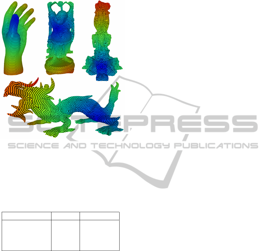
Figure 10: The Hand, the Happy Buddha, the Thai Statue
and Asian Dragon model with a distance field calculated
with the MDF.
Table 1: The MDF was performed on four different modes.
The average time for the MDF to visit the entire mesh surface
from
1000
different starting points was measured. Also
the distance difference for
1000
randomly picked pairs of
vertices where measured, when performing the calculation
twice by starting once from each vertex.
Model (# triangles)
Time [sec]
Length variation
Hand (76K)
0.11 0.115%
Happy (1.1M)
2.16 0.083%
Statue (10M)
23.5 0.112%
Asian Dragon (7.3M)
17.2
0.077%
on top of the MEF implementation, leaving poten-
tial for optimization. For instance the costly distance
calculation is done twice for every vertex, once for
anticipated distances, and again when actually adding
them to the front. This redundancy could be removed
by saving the initial calculation in another container.
The front-to-vertex calculation heuristic assumes that
the path from the current front to new vertices is al-
ways a straight line. This heuristic fails when two or
more triangles are passed which expose curvature. By
using the available
d
start
vectors to project the short-
est path onto those triangles the correct path could be
determined however.
Despite these imperfections the presented implementa-
tion of the MDF, when performed on different models
(see Fig. 10), calculates entire distance fields even for
meshes consisting of millions of triangles within sev-
eral seconds and distance calculations of the same path
on average differed in the one per mill range, as shown
in Table 1. Assuming this latter estimate represents
the actual distance error range, the approach would
come close to the accuracy of Surazhsky’s approach,
while not losing accuracy on complex models, such
as the Happy Buddha, as the FMM approach does
(these statements refer to the measurements presented
in (Surazhsky et al., 2005)). Additionally the approach
has major potential for runtime optimization.
Hardware:
Intel
R
Core 2 Extreme Quad Core
QX9300 (2.53GHz, 1066MHz, 12MB) processor with
8GB 1066 MHz DDR3 Dual Channel RAM. The algo-
rithm is not parallelized.
4 CONCLUSION
The presented edge-front data structures show great po-
tential for computer graphics applications. The edge
based front line allows differentiating many events,
such as collisions, and setting surface aspects in re-
lation to the front, such as the distance of vertices.
The edge-front also exploits the characteristics of a
2D surface to gain efficiency. Some extensions to the
edge-front model might be ”static edge path elements”
that do not expand, but confine the space in which the
edge-front expands. For instance, in the connection
path calculation the edge-fronts at the point when an
overlapping vertex is found could be saved. When cal-
culating the next recursive search level, the saved edge
path of the previous level could be used to confine the
search space making the search more efficient. A disad-
vantage of the edge-front data structure is its complex
implementation in comparison to vertex based front.
The focus of this paper was to present the edge-front
data structure. The geodesic calculations performed
with the MDF proved the potential of the presented
processing strategy. The data structure is virtually
parameter free and can easily be altered for individual
problem cases. It can be started from a point as well as
a line and it can deal with challenging triangulations
and meshes with boundaries.
Nevertheless the presented MDF is not yet a full-
fledged geodesic algorithm. In the presented form
the algorithm cannot be used for arbitrary positions
projected onto a mesh, but only for vertices. The same
holds when starting the algorithm from a line, only ex-
isting mesh edges can be used. To start from arbitrarily
shaped lines, as in (Bommes and Kobbelt, 2007), a
mechanism for adding the required edges to a mesh
would be needed. To calculate actual shortest distance
GRAPP2014-InternationalConferenceonComputerGraphicsTheoryandApplications
74

paths independent of the existing edges and triangles
of a mesh, the introduction of temporary vertices and
temporary edges into a mesh by the MDF could be con-
sidered. The necessary vectors
d
start
, which represent
the on-surface projected path back to the starting point,
are already available in the current implementation.
These changes would be required to fully compare the
edge-front based solution especially to other geodesic
algorithms which exceeds the scope of this paper.
When the MDF would be used for creating an unwrap-
ping for texturing or a surface segmentation, an alter-
native collision behavior might be reasonable. When
fronts would not merge at collision, but remain build-
ing a collision line instead, a MDF would always only
contain one single continuous edge front. Using the
collision line as a cutting line, a surface could be cut
into one single connected sheet to be fitted into a tex-
ture space. For this task it would also be sensible to
add curvature into the expansion selection process to
avoid flat surface regions from being cut.
REFERENCES
Annuth, H. and Bohn, C.-A. (2010). Smart growing cells.
In Proc. of the Int. Conf. on Neural Computation
(ICNC2010), pages 227–237. Science and Technology
Publications.
Annuth, H. and Bohn, C.-A. (2012). Resolving Twisted
Surfaces within an Iterative Refinement Surface Re-
construction Approach. In In Proc. of Vision, Modeling,
and Visualization (VMV 2012), pages 175–182.
Bommes, D. and Kobbelt, L. (2007). Accurate computation
of geodesic distance fields for polygonal curves on
triangle meshes. In Lensch, H. P. A., Rosenhahn, B.,
Seidel, H.-P., Slusallek, P., and Weickert, J., editors,
VMV, pages 151–160. Aka GmbH.
Bose, P., Maheshwari, A., Shu, C., and Wuhrer, S. (2011).
A survey of geodesic paths on 3d surfaces. Comput.
Geom. Theory Appl., 44(9):486–498.
Chen, J. and Han, Y. (1990). Shortest paths on a polyhedron.
In SCG 90: Proc. of the Sixth Annual Symposium on
Computational geometry, pages 360–369. ACM Press.
Crane, K., Weischedel, C., and Wardetzky, M. (2012).
Geodesics in heat. CoRR, abs/1204.6216.
Fritzke, B. (1993). Growing cell structures - a self-organizing
network for unsupervised and supervised learning.
Neural Networks, 7:1441–1460.
Hilaga, M., Shinagawa, Y., Kohmura, T., and Kunii, T. L.
(2001). Topology matching for fully automatic similar-
ity estimation of 3d shapes. In Proc. of the 28th annual
conference on Computer graphics and interactive tech-
niques, SIGGRAPH ’01, pages 203–212, New York,
NY, USA. ACM.
Ivrissimtzis, I. P., Jeong, W.-K., and Seidel, H.-P. (2003). Us-
ing growing cell structures for surface reconstruction.
In SMI ’03: Proc. of the Shape Modeling Int. 2003,
page 78, Washington, DC, USA. IEEE Computer Soc.
Kanai, T. and Suzuki, H. (2000). Approximate shortest path
on polyhedral surface based on selective refinement of
the discrete graph and its applications. In Proc. of the
Geometric Modeling and Processing 2000, GMP ’00,
pages 241–, Washington, DC, USA. IEEE Computer
Soc.
Kaneva, B. and O’Rourke, J. (2000). An implementation of
chen & han’s shortest paths algorithm. In CCCG.
Katz, S. and Tal, A. (2003). Hierarchical mesh decompo-
sition using fuzzy clustering and cuts. In ACM SIG-
GRAPH 2003 Papers, SIGGRAPH ’03, pages 954–961,
New York, NY, USA. ACM.
Kimmel, R. and Sethian, J. A. (1998). Computing geodesic
paths on manifolds. In Proc. Natl. Acad. Sci. USA,
pages 8431–8435.
Krishnamurthy, V. and Levoy, M. (1996). Fitting smooth
surfaces to dense polygon meshes. In SIGGRAPH,
pages 313–324.
Lanthier, M., Maheshwari, A., and Sack, J.-R. (1997). Ap-
proximating weighted shortest paths on polyhedral sur-
faces. In Proc. of the thirteenth annual symposium on
Computational geometry, SCG ’97, pages 485–486,
New York, NY, USA. ACM.
Mitchell, J. S. B., Mount, D. M., and Papadimitriou, C. H.
(1987). The discrete geodesic problem. SIAM J. Com-
put., 16(4):647–668.
Oliveira, G. N., Torchelsen, R. P., Comba, J. L. D., Walter,
M., and Bastos, R. (2010). Geotextures: A multi-
source geodesic distance field approach for procedural
texturing of complex meshes. In Proc. of the 2010
23rd SIBGRAPI Conf. on Graphics, Patterns and Im-
ages, SIBGRAPI ’10, pages 126–133, Washington,
DC, USA. IEEE Computer Soc.
Sethian, J. A. (1995). A fast marching level set method for
monotonically advancing fronts. In Proc. Nat. Acad.
Sci, pages 1591–1595.
Surazhsky, V., Surazhsky, T., Kirsanov, D., Gortler, S. J.,
and Hoppe, H. (2005). Fast exact and approximate
geodesics on meshes. In ACM SIGGRAPH 2005 Pa-
pers, SIGGRAPH ’05, pages 553–560, New York, NY,
USA. ACM.
Zigelman, G., Kimmel, R., and Kiryati, N. (2002). Texture
mapping using surface flattening via multidimensional
scaling. IEEE Trans. on Visualization and Computer
Graphics, 8(2):198–207.
GeodesicMeshProcessingwithEdge-FrontbasedDataStructures
75
