Peer Synchronization Method for Wireless Sensor Networks using

Heterogeneous Bluetooth Sensor Nodes

Steffen Dalgard, Franck Fleurey and Anders E. Liverud

SINTEF, Oslo, Norway

Keywords: Time Synchronization, Wireless Information Networks, Remote Sensing, Bluetooth, Bluetooth Smart,

Wireless Sensor Network.

Abstract: Synchronization of time is essential for correlation of sensor data. For body area network the sensors are

distributed over multiple sensor nodes located on different parts of the body. When collecting sensor data

using wireless sensor networks, the delay variation can be up to 1000 milliseconds. Physiological sensors,

like ECG, accelerometer and gyroscopes, require a timing accuracy in the millisecond range. This paper

describes a generic method to provide synchronized timestamps. The method is tested in a Wireless sensor

network using Bluetooth and Bluetooth Smart sensor nodes. Results show that the method is usable for

correlating sensor data with 50ms sample rate.

1 INTRODUCTION

Distributed multi sensor systems are gathering

physical measurements from multiple sensor nodes.

The measurements need to have a common timeline

for analysis and sensor fusion. Applications using

electrocardiogram (ECG), blood pressure sensors,

electromyography (EMG) and

accelerometer/gyroscopes often call for a timeline

with millisecond (ms) precision.

Wireless sensor networks are much used to

gather measurements from different sensor nodes in

distributed multi sensor systems. Sensor nodes

measure, process and transmit measurements to a

hub node for further analysis and data fusion. Each

measurement sample usually has timing information

attached, called timestamp.

If there is a predictable timing in the wireless

sensor network, the timestamp can be added at the

hub node. The hub node does usually have a time of

day clock reference that can be used for the

timestamp. However wireless sensor networks such

as Bluetooth don’t have deterministic timing

characteristics, both delays and delay variations are

unpredictable. This makes timestamp at millisecond

precision impossible to achieve when added at the

hub node.

Timestamp has to be added at the sensor node

doing the measurement to improve the accuracy.

This puts requirement on the sensor node to have a

synchronized clock with the hub node. Often the

sensor node is a highly integrated embedded

microcontroller with a free running clock counting

milliseconds since start-up. The processing capacity

is limited and there is no room for an additional time

of day clock component.

This paper introduces a method for achieving a

system synchronized timestamp from sensor nodes

realized using simple embedded microcontroller

with little processing and no need for additional

components. The method only use unicast peer

communication provided by all wireless sensor

networks. This enables the method to span different

network technologies when needed, making the

method useful for heterogeneous networks. The

implementation described in this paper shows this by

combining Bluetooth and Bluetooth Smart sensor

nodes in a synchronized system.

Relation to other synchronization methods is

presented in chapter 2. The method is described in

chapter 3. Implementation and test setup is described

in chapter 4. Results, conclusions and improvements

are presented in chapter 5 and 6.

2 CLOCK SYNCHRONIZATION

METHODS

Many synchronization methods are described in

175

Dalgard S., Fleurey F. and E. Liverud A..

Peer Synchronization Method for Wireless Sensor Networks using Heterogeneous Bluetooth Sensor Nodes.

DOI: 10.5220/0004696701750180

In Proceedings of the 3rd International Conference on Sensor Networks (SENSORNETS-2014), pages 175-180

ISBN: 978-989-758-001-7

 2014 SCITEPRESS (Science and Technology Publications, Lda.)

literature, and a thorough description can be found

in (Elson, 2003). Most of the methods are not easily

portable to embedded microcontrollers without

dedicated clock components. The accuracy for many

of the methods is in the microsecond range, making

the implementation costly. Broadcast protocols are

often used; this is generally not available for

Bluetooth.

Bluetooth systems do have a clock used as base

for the frequency hopping (312,5us) to synchronize

the different nodes. This is a very precise clock, but

few Bluetooth modules and protocol stacks provide

access to this clock through the application interface.

Clock synchronization methods using this clock can

be found in (Bluetooth 2009) and (Casas, 2005). The

method described in this paper use a peer protocol

and does not need access to the Bluetooth clock.

Network Time Protocol (NTP) (Mills, 2010) is

widely used for synchronizing computers in an IP-

network. Poll packets are sent over the network and

a number of time of day slave clocks are

synchronized to a time of day master clock through a

hierarchy. It is highly optimized to reduce the

number of poll packets sent which is important for

scalability. A poll rate slower than 10 minutes puts

requirement on active clock adjustments at each

slave to compensate for oscillator drift between each

poll. To implement NTP an additional clock

component is needed. The method described in this

paper does not need active clock adjustment of the

slave clock, and time of day clock functionality is

not needed. This simplifies the implementation of

the sensor node software and no additional clock

component is needed.

3 DESCRIPTION OF

SYNCHRONIZATION METHOD

The method is a peer protocol synchronizing a sync

master and a sync slave. The method is based on the

poll sequence as described in (Mills, 2010). The

goal is to calculate an offset value that can be used

to convert the slave timestamp to a master

timestamp. By adding the offset to the slave

timestamp, the timestamp is converted from slave

clock to master clock timeline (1).

The master initiates a poll sequence at regular

intervals. The slave is replying with its local slave

clock time when polled. The master will run the

offset calculator using equations (2) and (3),

calculating an offset between the two clocks based

on three time values; transmission of request (TMT)

and reception of reply (TMR) using master clock

and the time for reception of request at the slave

(TS) using local slave clock. This is a simplification

reducing the amount of data compared to (Mills,

2010) where the slave reply delay is added to (2).

This simplification is ok if slave response is

insignificant compared to other errors.

(TS

) = TS

+ Offset

(1)

= (TMR

– TMT

) / 2

(2)

Offset

= TMT

+ D

- TS

(3)

The transmission delay D is the time used for

sending the request from master to slave. It is

estimated to be half of the time between TMT and

TMR; hence symmetrical transmission delay is

assumed. Asymmetric delay is a significant error

source. The variance of the calculated offset (3) is

normally best for the lowest delays (2). By plotting

the calculated delay and offset from many poll

sequences in a XY-graph a statistical spread can be

analysed. See more about this in the result section.

More detailed information can be found in (Mills,

2010) and (Clock, 2012).

Each poll sequence produce a calculated offset

(Offset

) value based on (2) and (3). Due to delay

variation in the wireless network the calculated

offset will result in unacceptable large jitter. The

calculated offset from each poll sequence is fed

through a number of steps to calculate a

I-regulator

Offset calculator

(TMT

, TMR

, TS

Offset

)

Rejection filter

(Offset

)

  







   



/10





RegOffset

err

Poll sequence

Maste

Slave

TMT

TMR

Reply(TS

)

Request

TM(TS

)

Figure 1: Block diagram showing the steps used for calculating a stable RegOffset.

SENSORNETS2014-InternationalConferenceonSensorNetworks

176

sufficient stable offset (RegOffset). These steps are

shown in Figure 1 and described in the next

paragraphs.

A rejection filter evaluates each calculated offset

value to find whether it is usable for further

processing. Some values may be completely off

scale due to transient delays in the network. These

values have to be rejected. The accepted offset

values (Offset

) are fed into an I-regulator.

The I-regulator compares each accepted offset

value with the current stable offset (RegOffset). The

comparison is a feedback path that enables the

regulator to track the clock drift changes between

master and slave. The error is accumulated in the

regulator. The RegOffset value is calculated by

multiplying accumulated error with the integration

factor ki. RegOffset is calculated for each accepted

offset value, but its value will not change at each

calculation. The RegOffset changes so slowly that it

is usable for calculating timestamps using (4). Each

time a measurement is done its timestamp can be

converted using (4) at the cost of one integer

addition.

meas

(TS

meas

) = TS

meas

+ RegOffset (4)

To speed up the I-regulator at start-up, an initial

offset (ZeroOffs) is calculated. The average of the

first 10 accepted offset values is used. An average is

needed to compensate for the delay variation in the

network. When the ZeroOffset is calculated the rest

of the accepted offset values will be fed to the

comparator.

The poll rate together with the integration factor

ki decides the responsiveness of the regulator. The

integration factor ki can be in the (0,01..0,1) range in

order to integrate over 100 to 10 samples. A small ki

will use longer time to track, and this can be

observed as a constant lag error when oscillator drift

is large. The selection of ki decides the jitter, i.e.

change of RegOffset generated for each poll. A

monotonically increasing timestamp can be achieved

by having the RegOffset peak change less than half

the measurement sample rate.

The master can be implemented using integer

math. The integer size depends on the resolution and

timespan the implementation needs to cover.

The implementation of the master can be done at

the hub node or at the sensor node. Implementation

at the hub node will leave a minimum footprint at

the sensor node. The hub mode time format can be

invisible for the sensor node. This is convenient if

the sensor node needs to be time format agnostic. As

long as the number of master instances at the hub

node not causes problem, master at hub node is the

most flexible configuration.

Implementation of the master at the sensor node will

scale better for large configurations, where the hub

node gets measurements with ready calculated

timestamps. Equation (4) need to be reordered for

this configuration since TM needs to be converted to

TS.

4 IMPLEMENTATION AND

SETUP

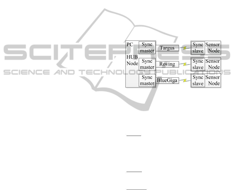
The experimental implementation described has a

PC as master and hub node and three embedded

microcontrollers as slaves and sensor nodes. The

setup is shown in Figure 2.

Figure 2: Setup with PC and three sensor nodes.

The master is implemented in Java running on a

MS Windows 7 PC. This is convenient for logging

of data for later analysis. Three sensor nodes using

different Bluetooth connections have been used;

Targus USB dongle with a Bluetooth host stack

running on the PC. Sensor node is using an ARM

CORTEX-M3 processors and a WT12 Bluetooth

module from BlueGiga running Serial Port Profile

(SPP) connected with a serial interface to the ARM

processor (Strisland, 2013).

Roving module with Bluetooth stack running on

module connected to the PC using FTDI serial

interface. Sensor node same as for Targus.

BlueGiga BLE112 USB dongle with Bluetooth

Smart stack running in the dongle. Sensor node is

using an ARM CORTEX-M3 processor and

nRF8001 Bluetooth Smart IC from Nordic

Semiconductor (Liverud, 2012).

The local clock for all sensor nodes is a crystal

producing 4ms ticks. All three sensor nodes have

been running simultaneously with various

measurements such as gyroscope and raw ECG. The

accuracy of the synchronization has been measured

by forcing a simultaneous rotation to the three nodes

and analysing the gyroscope measurements.

Poll sequence rate is set to 250 milliseconds and

PeerSynchronizationMethodforWirelessSensorNetworksusingHeterogeneousBluetoothSensorNodes

177

the integration factor ki is set to 1/64. Given an

ideal network without delay variation and total clock

drift at 50ppm, these parameters will give a constant

lag error at ~0,8ms. Delay variation in the network

will increase this error.

The prototype implementation of the master is

written in Java. Java is chosen for easy portability

between different operating systems and easy

distribution to different machines. The Java code is

available at (Open, 2013).

5 RESULTS

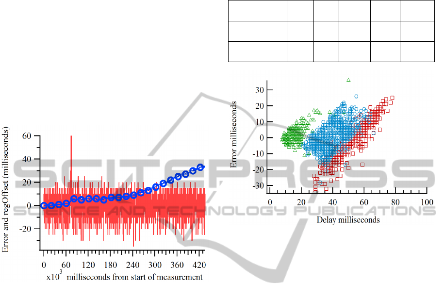
Figure 3: Error value (red line) fed to the integrator.

RegOffset value (blue circles) trend line delivered from

the regulator. Value shifted to zero at start of graph.

The RegOffset trend line in Figure 3 (blue line)

shows a typical trend over 7 minutes having 35ms

drift (35ms/7min => 83ppm). The error value fed to

the integrator in Figure 3 shows typical jitter on the

offset from each poll. There will be deviating polls

slipping through the rejection filter generating large

error values, but a ki=1/64 will attenuate these.

The tests show that the integration factor ki is

worth tuning. A low value results in low jitter for

RegOffset, but leads to long integration time. In our

experiment application there was a 4ms sample rate

and the jitter on the regOffset for one poll had to be

smaller than 2ms. A too large change in RegOffset

could produce timestamps out of sequence.

Table 1 shows jitter on RegOffset for different ki

values based on data using Targus dongle and one

sensor node. The values show that the jitter

produced by one poll could be in the range of 1ms

for ki less than 0,025 for a reasonable filter.

The formula for calculating the offset is based on

the assumption that the delay for request (DMS) and

Table 1: Jitter on RegOffset (milliseconds) for different ki

values based on data using Targus dongle and one sensor

node.

ΔRegOffset

(ms)

Ki=

0,1

Ki=

0,05

Ki=

0,025

Ki=

0,01

Ki=

0,005

1 poll max

min

3,3

-3,9

1,5

-1,9

0,8

-1,0

0,3

-0,4

0,2

-0,2

4 polls max

min

7,7

-7,2

3,8

-3,9

1,8

-2,1

0,7

-0,9

0,4

-0,4

Figure 4: Scatter diagram showing the spread of the

calculated error(offset) versus delay. Targus (blue circles),

Roving (red squares) and BlueGiga (green triangles).

reply (DSM) is symmetrical. The scatter diagram

Figure 4 is a x-y plot of the calculated delay and

error(offset) calculated by the offset calculator after

each poll sequence. The calculated offset is more

correct when the delay is low. A symmetrical delay

distribution should be a symmetric conical shape

with leftmost corner aligned at error=0.

Asymmetrical delays will result in other shapes with

an error offset. The error offset is a result of the I-

regulator behaviour that will average the spread

around error=0.

As shown in the diagram, each of the three

connections Targus, Roving and BlueGiga have very

different delay / offset distribution. Targus has a

fairly symmetrical distribution in the range 20-40ms

and an error offset of -5ms. Roving is not symmetric

at all and has an error offset of -30ms. BlueGiga has

symmetrical distribution and an offset of -1ms. The

error offset is important since it will cause a time

offset in conversion of the timestamps.

As a proof of concept we mounted the three

sensor nodes on a common bar. Data from the three

sensor nodes are flowing through each of the three

dongles to simulate different networks. By quickly

rotating the bar 180deg we could identify the

rotation in the gyroscope measurements and analyse

errors in the timing. The sample rate for the

SENSORNETS2014-InternationalConferenceonSensorNetworks

178

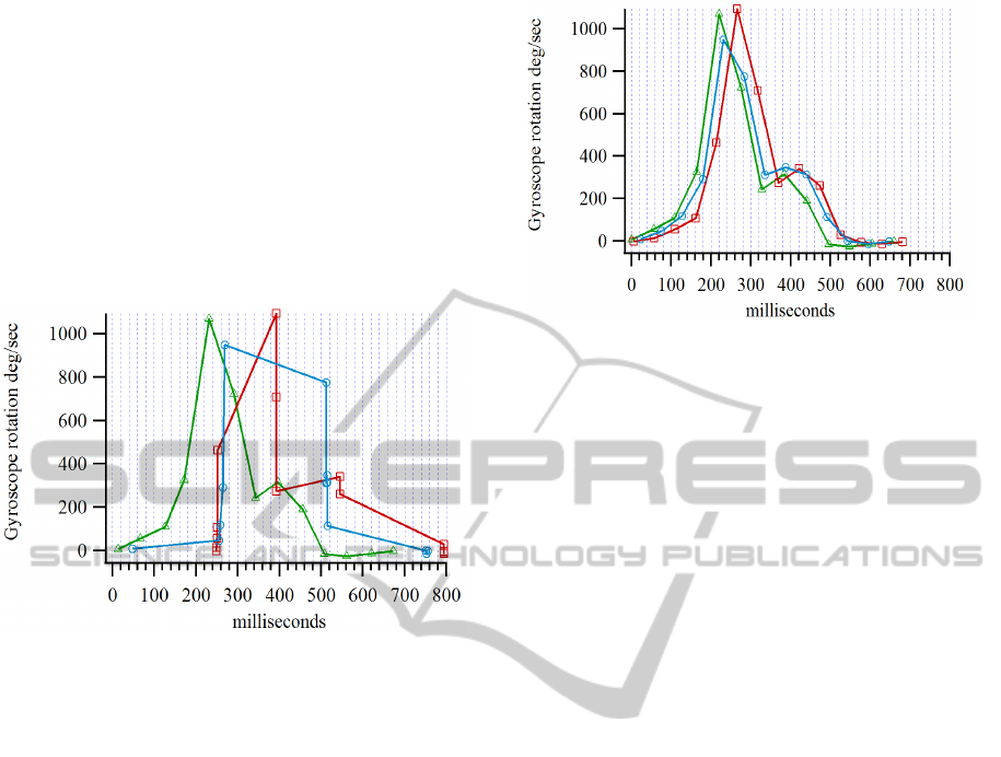
gyroscopes is 52 ms. Figure 5 shows gyroscope data

from the three sensor nodes. The data is plotted

using timestamp added by the hub node produced by

the Java application on the PC using the PC clock.

This is the typical approach without synchronized

clocks. The total plot spans over 800ms although the

rotation only last for 550ms. The plot shows that the

measurement data are shifted and chucked. Many

data samples at the same time are caused by buffers

emptied in bursts to the Java application. It is not

possible to see that they represent the same physical

rotation.

Figure 5: Gyroscope data from the three sensor nodes. The

data is plotted using the hub node reception timestamp in

ms produced by the Java application on the PC. Targus

(blue circles), Roving (red squares) and BlueGiga (green

triangles).

In Figure 6 the same data are plotted using

timestamp from the sensor nodes. The timestamp

values are calculated using (4). The result is

timestamps according to the PC clock. Now that the

timestamps are on a common timeline they can be

correlated. By comparing the two graphs the delay

for each sample can be deduced. Delays up to 200ms

are normal, and delays up to 1000ms are registered

during the experiment.

The time offsets between the Roving (red) and

Targus (blue) curves in Figure 6 are in the range of

25ms. Since these sensor nodes are identical, it is

reasonable to assume that the offset is due to the

different Bluetooth connections and the

synchronization method. The observed offset

correlates with the error offset that can be observed

in the scatter diagram Figure 4, where the red and

blue areas have an offset in the same range.

Experiments (not shown) with many sensor

nodes connected to the same Bluetooth dongle show

that the offset vs. delay spread has similar shape for

all sensor nodes. This results in a relative time offset

between the sensor nodes at about 10ms. This is

Figure 6: Gyroscope data from the three sensors. The data

is plotted using timestamp from the sensor nodes. Targus

(blue circles), Roving (red squares) and BlueGiga (green

triangles).

worth considering for homogenous networks.

6 CONCLUSIONS AND

DISCUSSION

The plot in Figure 6 shows that the synchronization

method is usable for correlating sample data with

50ms sample rate. This is sufficient for many

applications. The method both synchronizes and

tracks oscillator drift between the different clocks as

shown in Figure 3. The drift is typically in the 20-

100ppm range. The drift can vary over time due to

temperature changes. For a PC with temperature

controlled fan the drift will change when fan speed

changes.

The effects for the application are two fold,

firstly a proper timestamp is provided for each

sample from the sensor node. This enables multi

sensor data fusion for rapid changing signals.

Secondly, there is no need to optimize the hub node

software to make accurate timestamps. Such

optimization has shown to be hard for software

running on non-real-time systems as MS Windows

and Linux.

The effort adding synchronized timestamps for

sensor nodes is lowered by using the presented

method. Since the method is generic it can be

wrapped as a reusable object. The slave functionality

is only required to respond to the time request in the

poll sequence. By implementing the master at the

hub node the slave function can be implemented

with small effort at almost any sensor node with a

free running oscillator and a communication

channel.

PeerSynchronizationMethodforWirelessSensorNetworksusingHeterogeneousBluetoothSensorNodes

179

The method is tested in a non-homogenous network

using both Bluetooth SPP and Bluetooth Smart.

Since the method only uses unicast peer

communication it can be used in almost any network

system. This makes it flexible when combining

sensors from different vendors.

The poll rate can be made adaptable. The method

itself is not sensitive to poll rate or poll rate

deviation. It only integrates over available samples.

It is possible to have a high poll rate when

connecting and then reduce the rate when the

integrator has settled. The lag error due to the

oscillator drift will impose a lower limit for the poll

rate.

An additional shaping filter as the Huff-n'Puff

filter (Clock, 2012) used for asymmetrical delay

conditions may lower the observed offset shown in

the results. This may be used as an enhancement if

higher accuracy is needed in non-homogenous

networks.

ACKNOWLEDGEMENTS

The research leading to these results has received

founding from the European Commission as part of

the CORBYS (Cognitive Control Framework for

Robotic Systems) project under Seventh Framework

Programme contract FP7 ICT-270219. The views

expressed in this paper are those of the authors, and

not necessarily those of the consortium.

REFERENCES

Elson,Jeremy Eric, Time Synchronization in Wireless

Sensor Networks, 2003. University of California Los

Angeles http://lecs.cs.ucla.edu/~jelson/dissertation-

final.pdf.

Bluetooth SIG, Health Device Profile, Implementation

Guidance Whitepaper, 17 December 2009.

Casas R., et al., "Synchronization in Wireless Sensor

Networks Using Bluetooth,"in Intelligent Solutions in

Embedded Systems, 2005. Third International

Workshop on, 2005), pp.79-88.

Mills D. L., Network Time Protocol (version 4) Protocol

and Algorithm Specification, June. 2010, RFC-5905.

Martì Pau, Clock Synchronization for Networked Control

Systems Using Low-Cost Microcontrollers, Automatic

Control Department, Technical University of

Catalonia Research Report: ESAII-RR-08-02, 2008.

Clock Filter Algorithm (NTP) 14-Jun-2012

http://www.eecis.udel.edu/~mills/ntp/html/filter.html.

Strisland F,Svagård I, Seeberg T. M., Mathisen B. M.,

Vedum J, Austad H. O., Liverud A E., Kofod-Petersen

A., and Bendixen O. C., "ESUMS: A Mobile System

for Continuous Home Monitoring of Rehabilitation

Patients", Presented at EMBC 2013.

Liverud A. E, Vedum J, Fleurey F, and Seeberg T.M,

"Wearable Wireless Multi-parameter Sensor Module

for Physiological Monitoring," IOS Press, 2012, pp.

210-215.

Open source prototype implementation of the described

method named "rtsync" is available at

https://github.com/SINTEF-9012/rtsync.

SENSORNETS2014-InternationalConferenceonSensorNetworks

180