
Saliency Detection in Images using Graph-based Rarity, Spatial
Compactness and Background Prior
Sudeshna Roy and Sukhendu Das
Visualization and Perception Lab., Department of Computer Science and Engineering,
Indian Institute of Technology, Madras, India
Keywords:
Saliency, Spectral Clustering, Feature Rarity, Boundary Prior.
Abstract:
Bottom-up saliency detection techniques extract salient regions in an image while free-viewing the image.
We have approached the problem with three different low-level cues– graph based rarity, spatial compactness
and background prior. First, the image is broken into similar colored patches, called superpixels. To measure
rarity we represent the image as a graph with superpixels as node and exponential color difference as the
edge weights between the nodes. Eigenvectors of the Laplacian of the graph are then used, similar to spectral
clustering (Ng et al., 2001). Each superpixel is associated with a descriptor formed from these eigenvectors
and rarity or uniqueness of the superpixels are found using these descriptors. Spatial compactness is computed
by combining disparity in color and spatial distance between superpixels. Concept of background prior is
implemented by finding the weighted Mahalanobis distance of the superpixels from the statistically modeled
mean background color. These cues in combination gives the proposed saliency map. Experimental results
demonstrate that our method outperforms many of the recent state-of-the-art methods both in terms of accuracy
and speed.
1 INTRODUCTION
Visual Saliency have now a days become very pop-
ular and relevant way to deal with a lot of computer
vision tasks like object detection, object recognition,
content based image retrieval, scene understating etc.
It reduces the search space of the problem, as well
as helps in extracting correct features for these tasks.
It is a perceptual quality of the human visual system,
by which humans attend to a subset of the pool of
available visual information. Saliency of an image
is given by a saliency map where we assign a nor-
malized value to an image component or superpixel
denoting its probability of being salient. A salient
region in an image is sufficiently distinct from its
neighborhood in terms of visual attributes or features,
and grabs attention. In this paper, we concentrate on
unsupervised bottom-up saliency detection technique
when free-viewing a scene. Bottom-up saliency can
be thought as a filter which extracts selected spatial
locations of interest which generally stands out from
other locations. Most work in the past have defined
saliency by, either using spatial features like color,
orientation, spatial distances between image patches
(Itti et al., 1998), (Goferman et al., 2010), (Cheng
et al., 2011), (Perazzi et al., 2012), or using spec-
tral features like amplitude, phase spectrum (Hou and
Zhang, 2007), (Achanta et al., 2009), (Li et al., 2013),
(Schauerte and Rainer, 2012) and image energy in the
spectral domain (Hou et al., 2012) or graph based
method (Harel et al., 2006). Most of them have de-
fined saliency as rarity of occurrence (or as a sur-
prise) with respect to different local and global fea-
tures. Color difference in CIELab space is the most
distinctive feature which is used across most of the
models. Our spectral clustering based rarity and spa-
tial compactness measures of saliency exploit rarity
of feature to extract salient regions in an image.
Spectral clustering (Ng et al., 2001) is used in
many different applications like, page ranking (Zhou
et al., 2004), contour detection (Arbelaez et al., 2011),
normalized cut (Shi and Malik, 2000) approaches. A
recent paper (Yang et al., 2013) uses the ranking al-
gorithm (Zhou et al., 2004) to find salient regions in
images. We do not use any ranking technique (Zhou
et al., 2004) or like any Normalized Cut approach, we
do not cluster the descriptors obtained from the eigen-
vectors of the graph Laplacian. Instead, we find the
rarity using these descriptors itself, since eigenvectors
themselves carry information about the superpixels.
523
Roy S. and Das S..
Saliency Detection in Images using Graph-based Rarity, Spatial Compactness and Background Prior.
DOI: 10.5220/0004693605230530
In Proceedings of the 9th International Conference on Computer Vision Theory and Applications (VISAPP-2014), pages 523-530
ISBN: 978-989-758-003-1
Copyright
c
2014 SCITEPRESS (Science and Technology Publications, Lda.)

Along with the above measures, we exploit the
concept of background prior which is same as bound-
ary prior and connectivity prior (Wei et al., 2012)
concept. In this paper, background refers to the non-
salient spatial locations in the image. The main idea is
that, the distance between background patches will be
less and that between background and a salient patch
will be more. Recent, cognitive science literature
(Tatler, 2007) gives the evidence of boundary prior
and shows human fixation happens mostly at the cen-
ter. This motivates our second component of saliency
detection where we statistically model the boundary
patches of an image and use them as background
prior in a complete unsupervised formulation to de-
tect saliency. We call our proposed method which
is based on Graph-based Rarity, Spatial Compactness
and Background Prior, as PARAM (background Prior
And RArity for saliency Modeling).
2 RELATED WORK
Bottom up saliency models are mostly inspired by
neurophysiology, which adapt the concepts of feature
integration theory (FIT) (Tre, ) and visual attention
(Koch and Ullman, 1987). Itti et al.’s (Itti et al., 1998)
model uses three features, color, intensity and orien-
tation, like the simple cells in primary visual cortex.
Most computational models are based on either spa-
tial or spectral processing. Spatial models use differ-
ent local or global features, like color, intensity, spa-
tial distance, or a combination. Spectral models use a
spectral domain analysis of the image and inherently
use global features.
Among spatial models, Goferman et al. (Gofer-
man et al., 2010) model saliency using both local low-
level features and global considerations, as well as vi-
sual organization rules and high level features. They
have taken overlapping patches at different scales
and modeled saliency as distance in color, inversely
weighted by distance in position among the patches.
As a result, edges of the salient regions are high-
lighted more. Cheng et al. (Cheng et al., 2011)
have proposed a region-wise contrast based method
to compute saliency and uses GrabCut algorithm to
give a refined saliency cut. Being a global con-
trast based method, it works well for only large-scale
salient regions. Perazzi et al. (Perazzi et al., 2012)
divide the image into superpixels, computes saliency
using uniqueness and distribution properties and up-
samples it to gives a smooth, pixel-wise accurate
salient region. It gives a good precision for focused,
large salient regions but fails for small salient regions
and also for cluttered background. A recent method
(Yang et al., 2013) uses a spectral clustering based
ranking algorithm to rank the superpixels according
to their saliency, or precisely get the saliency proba-
bility values. Harel et al.’s model (Harel et al., 2006)
although fails to detect the entire salient object, works
comparatively well for multiple salient regions. But,
it gives a blurred map with less precision.
Among spectral analysis models, Hou and Zhang
(Hou and Zhang, 2007) represent a log spectrum and
Gaussian smoothed inverse Fourier transformed spec-
tral component for saliency. They use only the phase
information and thus works better for small salient re-
gions in an uncluttered background (Li et al., 2013).
Achanta et al. in their model (Achanta et al., 2009)
first omit the very high frequency components as
those correspond to background texture or noise arti-
facts and then computes saliency as the distance from
mean color in Lab color space. A more advance
model (Li et al., 2013) uses hypercomplex Fourier
transform (HFT) over different features like (Itti et al.,
1998) and does a spectrum scale space analysis. Opti-
mal scale is detected by minimizing an entropy, with
saliency as probability maps. It gives good results
for images with different sizes of salient regions with
varying background, but results are blurred and fails
to give accurate object boundary. Hou et al. in (Hou
et al., 2012) prove that Inverse Discrete Cosine Trans-
form (IDCT) of the sign of DCT of an image, con-
centrates the image energy at the location of spatially
sparse foreground. This holds good for only small and
sparse salient regions.
In this paper, we propose a novel unsupervised
formulation of saliency measure using appropriate
features for discriminating the salient region from the
background. Features are based on color and spatial
distance of superpixels. Graph based (spectral clus-
tering) rarity approach uses eigenvectors of the Lapla-
cian of the affinity graph. The spatial compactness
term is a modified version of the distribution term of
(Perazzi et al., 2012). The other component is color
divergence with respect to the patches at the border
of an image. (Wei et al., 2012) uses the concept
in a semi-supervised algorithm which requires man-
ual intervention. We statistically model the boundary
patches using Gaussian Mixture Model (GMM), and
find the distance of all the patches from the modeled
background colors in Lab color space. Integration of
these priors gives the saliency map.
VISAPP2014-InternationalConferenceonComputerVisionTheoryandApplications
524
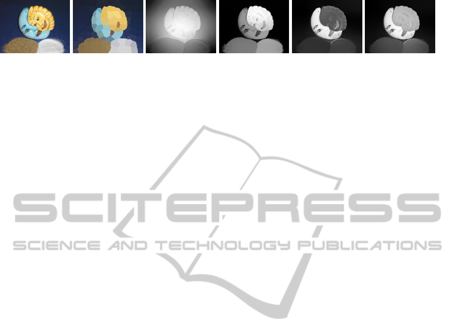
(a)
(b) (c) (d) (e) (e)
Figure 1: (a) Image; (b) Superpixels; (c)Saliency by Graph-based rarity; (d) Spatial compactness; (d) Background prior and
(e) Proposed Saliency Map.
3 BRIEF OVERVIEW OF OUR
APPROACH
3.1 Abstract the Image into Superpixels
We first break our image into superpixels using
SLIC superpixel (Achanta et al., 2010) method which
makes our method computationally fast. All compu-
tations are hence performed on superpixels which are
much lesser in number than the set of pixels. Each su-
perpixel is represented by a 5-D vector {labxy}. Thus
each patch has its specific color and position.
3.2 Graph-based Spectral Rarity
We use the eigenvectors of the normalized Lapla-
cian matrix of the affinity graph with superpixels as
nodes. If we look closely, the laplacian matrix pro-
vides a measure of the fraction of time a free random
walker would spend at each node and what are the
most preferable nodes to go from a particular node,
considering the edge weights as cost of moving from
one node to the other. Hence, as also mentioned by
(Arbelaez et al., 2011), this carries information about
the edges in the image. If a random walker has little
probability to move from a particular node to another,
there is an edge in the image between the two super-
pixels. The descriptor extracted from the eigenvectors
of the normalized Laplacian matrix, when using su-
perpixels as nodes, would capture the corresponding
coarse texture information. Hence, local and global
rarity based on these descriptor would give a measure
of saliency which takes rarity of textures into account.
3.3 Spatial Compactness
We exploit the fact that a salient object would be spa-
tially compact and the background colors will be dis-
tributed over the whole image (Goferman et al., 2010)
(Hou and Zhang, 2007). As, human eye can fixate at
only one position and vision is centre surround, spa-
tial compactness is an important characteristics of an
object to become salient. So, the color belonging to
the salient object will be spatially clustered together.
Whereas, colors belonging to background will have
high spatial variance. Hence, we use spatial variance
of color or color compactness as a measure of saliency
detection. The less the spatial variance more compact
the object is and thus more salient.
3.4 Background Prior
However, rarity of feature alone is not sufficient to
detect saliency, as some previous methods in litera-
ture (Perazzi et al., 2012)(Cheng et al., 2011) show.
We exploit the concept of boundary prior (Wei et al.,
2012), which comes from the natural fact that bound-
ary of an image would be mostly occupied by back-
ground (Tatler, 2007). Moreover, background will
be mostly spatially distributed but homogeneous (in
parts, say, the sky above and the grass below, for a
natural scene) which results in compact clusters in
color (feature) space. Hence, distance between these
background patches will be less, but background and
fore-ground salient patches will be high, in 3-D Lab
color space. However, occasionally a part of the
salient object may exists at the boundary. Hence, it
is not justified to consider all the boundary patches
as background. To solve this, we statistically model
the boundary patches using GMM. Here, Gaussian
modes with large number of pixels, having a large
value of mixture coefficient, will generally model the
background colors. Whereas, some Gaussian modes
which model the few salient object patches, present at
the image boundary, will naturally have low mixture
coefficient. Hence, we exploit Mahalonobis distance
in color space, between the image patches and these
modes, weighted by the corresponding mixture coef-
ficients, to computed a good measure of saliency.
3.5 Pixel Accurate Saliency
Finally, we combine the saliency measures yielding a
granulated saliency map at superpixel level. To get a
pixel accurate saliency map we use the up-sampling
technique proposed by (Dolson et al., 2010)(Perazzi
et al., 2012).
SaliencyDetectioninImagesusingGraph-basedRarity,SpatialCompactnessandBackgroundPrior
525

Results of individual components are illustrated
in the Figure 1 and shows it finally produces an im-
proved saliency map.
4 ALGORITHM FOR SALIENCY
MAP ESTIMATION
We formulate two new measures of saliency detec-
tion, using graph-based rarity, spatial compactness of
color and statistical model of boundary colors. The
overall process of saliency computation is described
in the following subsections:
4.1 Pre-processing
We first represent the image using superpixels by ex-
ploiting the concept of SLIC superpixel segmentation
(Achanta et al., 2010) in five-dimensional {labxy}
space. We input the number of clusters as 400, for
all the experiments, to the SLIC superpixel algorithm
which yields N superpixels. The benefit of SLIC seg-
mentation is that, it produces compact homogeneous
color patches as clusters. This helps the next stages of
our algorithm. Each superpixel, i has color in CIELab
space c
i
and position p
i
. In the following subsection,
we describe the measures for saliency computation.
4.2 Saliency Computation
Our measure of saliency has broadly two components
for salient object detection. The first one is given by
graph-based spectral rarity and spatial compactness
of the salient object. This approach exploits rarity of
feature. Whereas, the second component of saliency
detection utilizes the concept of boundary prior and
connectivity prior (Wei et al., 2012).
4.2.1 Graph-based Spectral Rarity
Given an image we define a graph G = (V, E)
whose nodes are the superpixels and edges E are
weighted by an affinity matrix W = [w
i j
]
NXN
. Let
D = diag{d
11
, ..., d
NN
}, where d
ii
=
∑
j
w
i j
. Then
Laplacian of the graph G, can be given by L = I −
D
−
1
2
W D
−
1
2
. Let, {v
1
, ..., v
k
} are the eigenvectors cor-
responding to largest k eigenvalues of L. We form the
matrix X
N×k
by stacking the eigenvectors in columns.
Now we take normalized row vectors of X
N×k
as the
descriptor for each superpixel. Let the k-dimensional
descriptors are {x
1
, ..., x
N
} and position of superpixel
i is p
i
. We find rarity of the i
th
superpixel using the
following formulation,
r
i
=
N
∑
j=1
||x
j
− x
i
||
2
exp(−k
r
||p
j
− p
i
||
2
) (1)
where, ||.|| implies Euclidean distance. k
r
is the fac-
tor that controls how much local the rarity is. If k
r
is infinite, it becomes a global rarity measure. k
r
is
set to 8.0 in all the experiments. We take the weight
between two nodes, w
i j
= exp(−||c
i
− c
j
||
2
), i, j ∈ V .
Figure 1 (b) shows the saliency map generated using
only r
i
as saliency probability of i
th
superpixel.
4.2.2 Spatial Compactness
We define spatial variance of color (v
i
) of a super-
pixel i, with color in CIELab space c
i
and position p
i
as, how much similar colored patches are distributed
over the image. A salient color is expected to be spa-
tially compact and thus will be close to the spatial
mean position of the particular color (Perazzi et al.,
2012). Thus, v
i
is computed as,
v
i
=
N
∑
j=1
||p
j
− µ
i
||
2
. exp(−k
c
||c
j
− c
i
||
2
) (2)
where, µ
i
, the weighted mean position of color c
i
,
gives the mean position of a particular color, c
i
,
weighted by the difference in color with other simi-
lar colored patches, as
µ
i
=
Σ
N
j=1
p
j
. exp(−k
c
||c
j
− c
i
||
2
)
Σ
N
j=1
exp(−k
c
||c
j
− c
i
||
2
)
(3)
k
c
controls the sensitivity of color similarity while
computing their spatial mean position. k
c
is set as
in (Perazzi et al., 2012) in all the experiments. High
value of k
c
implies that, only when the colors of the
patches are very similar, it would contribute to the
computation of µ for that particular color.
If the spatial variance of color for superpixel i is less,
it corresponds to a salient region, and not the back-
ground, as background colors are generally dispersed
over the entire image. Thus, for a salient superpixel
i, its mean (µ
i
) will be spatially near to, p
i
and also
to all the p
j
s belonging to similar colored patches in
2-D spatial space. And only the patches, for which
c
j
' c
i
will contribute to the term v
i
. So, for a salient
patch i, v
i
will be small as p
j
s are close to µ
i
mak-
ing ||p
j
− µ
i
|| small ∀ j|c
j
' c
i
. Hence, The lower the
value of v
i
, the more salient is the region i.
Hence, our first component of saliency for i
th
su-
perpixel using feature rarity is given as,
F
i
= exp (−k.v
i
).r
i
(4)
VISAPP2014-InternationalConferenceonComputerVisionTheoryandApplications
526
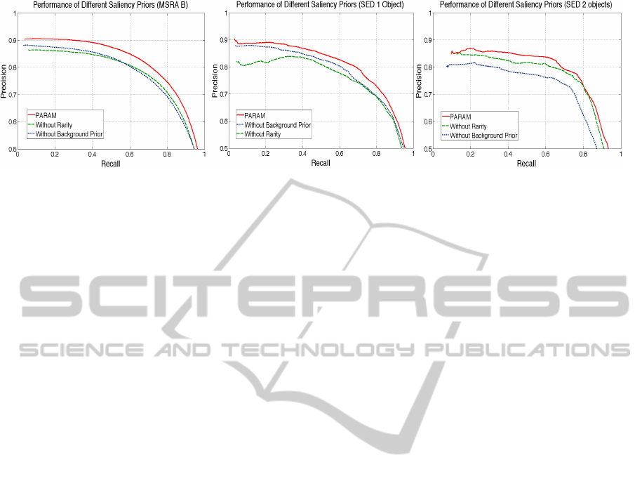
(a)
(b)
(c)
Figure 2: Performance curve illustrating the importance of the different components of our method (PARAM) for saliency
computation using Precision vs Recall metric on: (a) MSRA B; (b) SED1 and (c) SED2 Datasets.
Figure 1 (c) shows the saliency map generated using
only exp(−k.v
i
) as saliency probability of i
th
super-
pixel. Large value of F
i
indicates greater saliency. k
is the scale of the exponent and set to 3 in all the ex-
periments, as in (Perazzi et al., 2012).
4.2.3 Background Prior
The above feature rarity based method is not enough
to find salient object in all different types of im-
ages, specially with small or more than one salient
objects. We assume that boundary superpixels are
less likely to be salient and recent studies in cog-
nitive science (Tatler, 2007) reveals the same. This
criteria is derived from prior observation of samples
from various benchmark datasets, and requirements
of saliency in many application domains (CBIR, ob-
ject recognition, target acquisition etc.). We model
the boundary superpixels using a Gaussian Mixture
Model (GMM) in CIELab-color space and find the
Mahalanobis distance (D
M
) of all the superpixels
from the Gaussians means. The more a superpixel
differs in Lab-color space from the boundary super-
pixels, more is its saliency. Whereas, background su-
perpixels are mostly homogeneous and thus distance
of background patches from these GMM means will
lesser. Again, boundary is mostly occupied by non-
salient background superpixels. So, more the value of
mixture coefficient (π
j
) of a GMM component, more
likely that the component refers to a non-salient color.
Following above, the second component of
saliency measure of i
th
superpixel, using background
prior is formulated as,
B
i
=
K
∑
j=1
π
j
.D
M
(c
i
, µ
G j
) (5)
where, D
M
(x, y) denotes Mahalanobis distance be-
tween x and y, c
i
is the color of i
th
superpixel, µ
G j
is the mean of jth Gaussian mode, π
j
is the weight
or mixture coefficient of the j
th
Gaussian and K is
the number of GMM components used to model the
distribution of the boundary superpixels in CIELab
space. We dynamically compute the optimal value of
K maximizing the cluster compactness of the bound-
ary patches. Figure 1 (d) shows the saliency map gen-
erated using B
i
as saliency probability of i
th
super-
pixel.
4.3 Saliency by Up-sampling to Image
Resolution
Saliency of each pixel is taken as a weighted linear
combination of saliency of its surrounding image ele-
ments, S
j
, using the idea proposed by (Dolson et al.,
2010). In our work, S
j
, the saliency value of j
th
patch,
is sum of F
j
and B
j
and we use the same formulation
as used in (Perazzi et al., 2012).
Figure 2 shows the contribution of the saliency
priors. It shows the performances by excluding r
i
from eq. 4 and without background prior concept
(eq. 5), that is only exploiting eq. 4, along with fi-
nal saliency map (PARAM), on different datasets (for
details of experimentation see Section 5.2).
5 RESULTS AND
PERFORMANCE EVALUATION
5.1 Datasets
We evaluate the performance of our proposed
method (PARAM) using the following two benchmark
datasets.
SaliencyDetectioninImagesusingGraph-basedRarity,SpatialCompactnessandBackgroundPrior
527
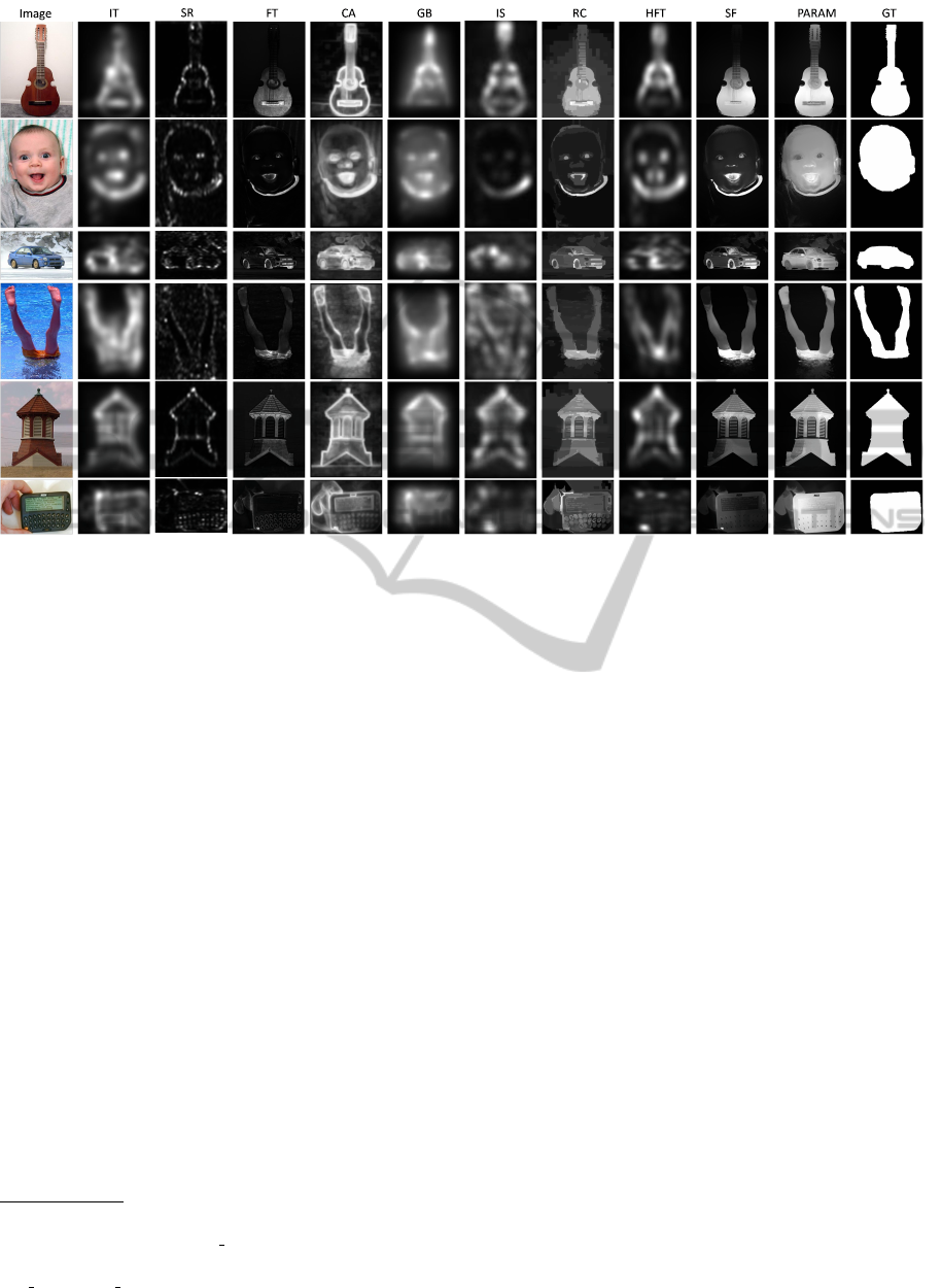
Figure 3: Visual comparison of the results of nine state-of-the-art methods along with our proposed method (PARAM) of
saliency estimation on six different samples of MSRA B dataset. PARAM consistently performs better for different types of
images including indoor, outdoor natural scenes, when compared with the ground truth given in the last column.
5.1.1 MSRA B
1
MSRA B has 5000 images with their ground truth
masks as given in the papers, (Achanta et al., 2009)
and (Jiang et al., 2013). Images are of numerous kind
including indoor, outdoor natural scenes, humans, an-
imals with different types of contrast and color vari-
ance. This makes the dataset diverse and challenging.
5.1.2 SED
2
Segmentation Evaluation Dataset (SED) has two
parts, SED1 and SED2. SED1 has 100 images with
a single salient object. SED2 images has 100 images
with 2 different salient objects of different size and
color. Ground truth masks for all the images are pub-
licly available.
5.2 Experimentation
We compare the performance of our proposed
method, PARAM, with 9 state-of-the-art methods, IT
(Itti et al., 1998), SR (Hou and Zhang, 2007), CA
(Goferman et al., 2010), FT (Achanta et al., 2009),
1
http://research.microsoft.com/en-us/um/people
/jiansun/SalientObject/salient object.htm
2
http://www.wisdom.weizmann.ac.il/∼vision/
Seg Evaluation DB/dl.html
RC (Cheng et al., 2011), IS (Hou et al., 2012), GB
(Harel et al., 2006), HFT (Li et al., 2013), SF (Perazzi
et al., 2012).
Figures 3 - 6 show results of these 9 different state-
of-the-art saliency detection methods along with our
proposed method, PARAM. Results in Figure 3 visu-
ally illustrates that the saliency map provided by our
method (PARAM) is closest to the ground truth (de-
noted by GT) and highlights the overall salient object
uniformly, giving better result than the existing state-
of-the-art methods.
5.2.1 Quantitative Performance Evaluation
We quantitatively evaluate the performance of our
method (PARAM) using precision, recall rate similar
to the (Achanta et al., 2009), (Cheng et al., 2011),
(Hou and Zhang, 2007). We generate the precision-
recall curve by producing binary maps at different
thresholds similar to (Achanta et al., 2009). We
have compared our method with all the above men-
tioned 9 state-of-the-art methods. We do not com-
pare with (Jiang et al., 2013), as being a training
based method it has output for only 2000 images. Our
method, PARAM clearly out-performs all the methods
on MSRA B (Figure 4 (a)) and SED1 (Figure 4 (b))
datasets. On SED2 (Figure 4 (c)) dataset, PARAM is
not a clear winner. This is mainly due to the occa-
VISAPP2014-InternationalConferenceonComputerVisionTheoryandApplications
528
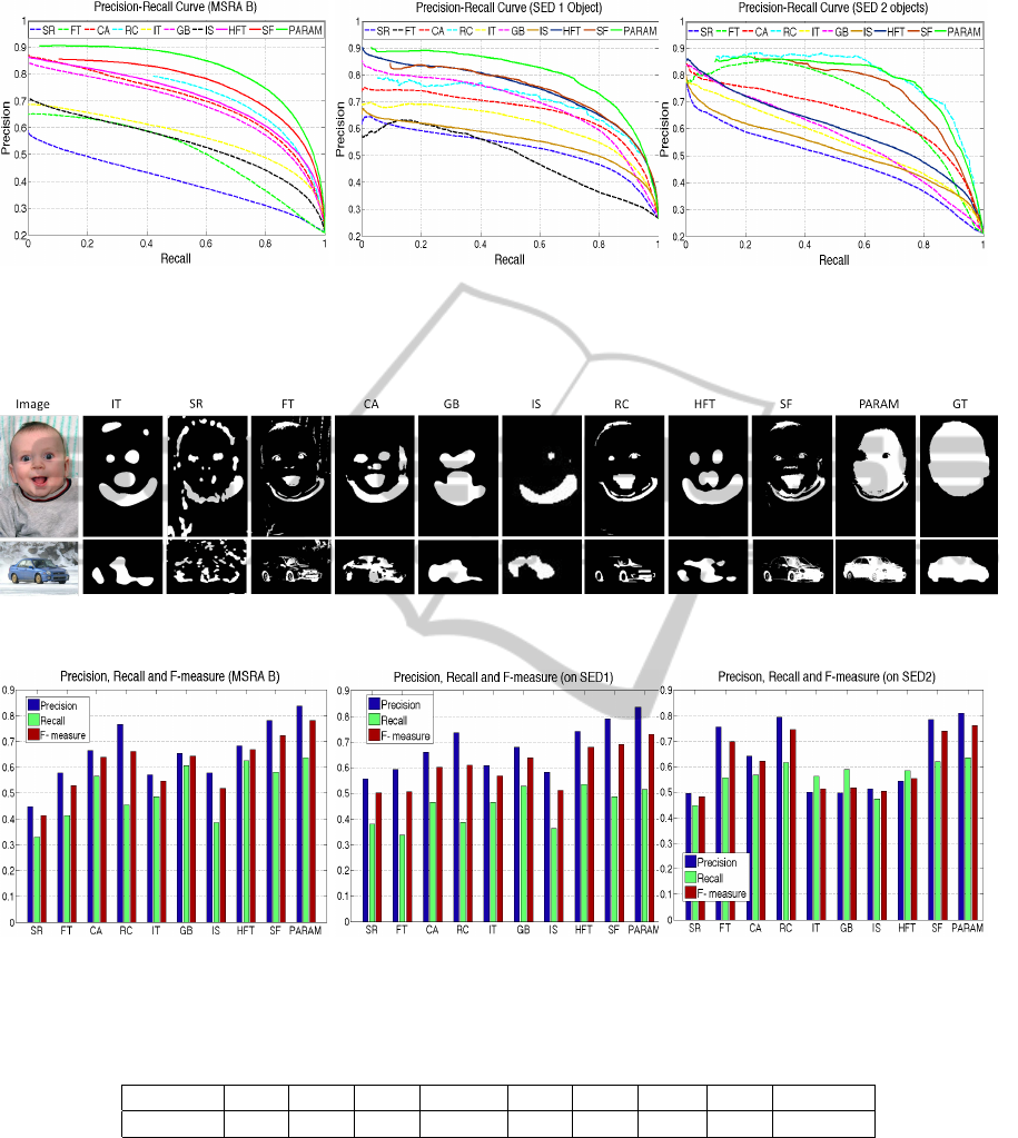
(a)
(b)
(c)
Figure 4: Performance analysis of 9 different state-of-the-art methods along with our proposed method (PARAM) using
Precision vs Recall metric on: (a) MSRA B; (b) SED1 and (c) SED2 Datasets. It shows that our method performs over all the
best on MSRA B as well as both the SED datasets. This figure is best viewed in color.
Figure 5: Visual comparison of the Adaptive Cut binary maps of the nine state-of-the-art methods and our proposed method
(PARAM) on two samples of MSRA B dataset, with the ground truth as given in the last column.
(a) (b)
(c)
Figure 6: Precision, Recall & F-measure using adaptive cut on (a) MSRA B; (b) SED1 and (c) SED2 datasets, show that our
method (PARAM) performs better than all the 9 state-of-the-art methods for all the datasets.
Table 1: Average runtime (in seconds per image) of different competing methods.
Method IT FT GB CA RC IS HFT SF PARAM
Time (s) 0.41 0.13 1.63 128.05 0.21 2.20 0.76 0.23 0.23
sional presence of two objects only on the boundary.
Such a scenario is not biologically plausible to be-
come salient for human vision.
We take the adaptive threshold as twice of average
saliency and create a binary map, which is proposed
as Adaptive Cut in (Achanta et al., 2009). Figure
5 shows the binary maps or adaptive cuts which are
generated using adaptive threshold, from the saliency
maps obtained from the 9 different state-of-the-art
and our proposed method, PARAM. From these binary
maps we calculate specific values of precision, recall
and the f-measure as in (Achanta et al., 2009), for the
9 methods along with PARAM. The bar charts in Fig-
ure 6 show that PARAM produces the best result for
all the three performance measures: Precision, Recall
and F-measure.
SaliencyDetectioninImagesusingGraph-basedRarity,SpatialCompactnessandBackgroundPrior
529

5.2.2 Efficiency
Although our method has different saliency priors,
it is time efficient and can be easily used as prepro-
cessing step for different applications. This is mainly
due to the fact that the saliency computation by our
method is performed on image patches or superpix-
els which are much lesser in number than the set of
pixels. Moreover, parallel computation of the priors
is also possible. We compare the running time of our
implementation (in C++) with other competing meth-
ods. We use Matlab implementation from authors for
(Itti et al., 1998), (Goferman et al., 2010), (Achanta
et al., 2009), (Li et al., 2013), (Harel et al., 2006),
(Hou et al., 2012) and C++ implementation of (Cheng
et al., 2011), (Perazzi et al., 2012) on a intel core 2
extreme 3.00 GHz CPU with 4 GB RAM. Table 1
lists the average running time of 8 competing methods
along with PARAM. For (Hou and Zhang, 2007) we
get the results from the publicly available executable
of (Cheng et al., 2011), and we do not have the time
efficiency information for the same. The work pro-
posed in (Achanta et al., 2009) is the fastest, but per-
forms much inferior (refer Figures 3 - 6).
6 CONCLUSIONS
We have presented a bottom-up saliency estimation
method for images using low level cues. We have
proposed a novel graph-based feature rarity computa-
tion, utilizing the concepts of spectral clustering (Ng
et al., 2001). It shows that eigenvectors of Laplacian
of the affinity matrix of the graph, taking image ele-
ments as node gives good measure of rarity. Again,
we exploit spatial compactness of color and we use
the cue of boundary prior by statistically modeling
the background in color space. We show, both quali-
tatively (Figure 1) and quantitatively using Precision-
Recall metric (Figure 2), that these components com-
pliment each other. We also give a comparative study
of the performance of our method with 9 state-of-the-
art methods, using three different measures of evalu-
ation on two popular real-world benchmark datasets.
Since, our method is not just restricted to global spa-
tial feature rarity, but also utilizes the boundary cue as
well as spectral clustering based feature rarity, it gives
better performance and in most of the cases accurately
detects the salient object.
REFERENCES
A feature-integration theory of attention. Cognitive Psy-
chology, 12(1).
Achanta, R., Hemami, S., Estrada, F., and Susstrunk, S.
(2009). Frequency-tuned salient region detection. In
CVPR.
Achanta, R., Shaji, A., Smith, K., Lucchi, A., Fua, P., and
Susstrunk, S. (2010). SLIC Superpixels. Technical
report, EPFL.
Arbelaez, P., Maire, M., Fowlkes, C., and Malik, J. (2011).
Contour detection and hierarchical image segmenta-
tion. TPAMI, 33(5):898–916.
Cheng, M.-M., Zhang, G.-X., Mitra, N. J., Huang, X., and
Hu, S.-M. (2011). Global contrast based salient region
detection. In CVPR.
Dolson, J., Jongmin, B., Plagemann, C., and Thrun, S.
(2010). Upsampling range data in dynamic environ-
ments. In CVPR.
Goferman, S., Zelnik-manor, L., and A.Tal (2010). Context-
aware saliency detection. In CVPR.
Harel, J., Koch, C., and Perona, P. (2006). Graph-based
visual saliency. In NIPS, pages 545–552.
Hou, X., Harel, J., and Koch, C. (2012). Image signature:
Highlighting sparse salient regions. TPAMI, 34(1).
Hou, X. and Zhang, L. (2007). Saliency detection: A spec-
tral residual approach. In CVPR, pages 1–8.
Itti, L., Koch, C., and Niebur, E. (1998). A model of
saliency-based visual attention for rapid scene anal-
ysis. TPAMI, 20(11).
Jiang, H., Wang, J., Yuan, Z., Wu, Y., Zheng, N., and Li,
S. (2013). Salient object detection: A discriminative
regional feature integration approach. In CVPR.
Koch, C. and Ullman, S. (1987). Shifts in selective visual
attention: Towards the underlying neural circuitry. In
Matters of Intelligence, volume 188. Springer Nether-
lands.
Li, J., Levine, M. D., An, X., Xu, X., and He, H. (2013).
Visual saliency based on scale-space analysis in the
frequency domain. TPAMI, 35(4).
Ng, A. Y., Jordan, M. I., and Weiss, Y. (2001). On spectral
clustering: Analysis and an algorithm. In NIPS, pages
849–856.
Perazzi, F., Krahenbuhl, P., Pritch, Y., and Hornung, A.
(2012). Saliency filters: Contrast based filtering for
salient region detection. In CVPR.
Schauerte, B. and Rainer, S. (2012). Quaternion-based
spectral saliency detection for eye fixation prediction.
In ECCV, pages 116–129.
Shi, J. and Malik, J. (2000). Normalized cuts and image
segmentation. TPAMI, 22(8):888–905.
Tatler, B. W. (2007). The central fixation bias in scene view-
ing: Selecting an optimal viewing position indepen-
dently of motor biases and image feature distributions.
Journal of Vision, 7(14).
Wei, Y., Wen, F., Zhu, W., and Sun, J. (2012). Geodesic
saliency using background priors. In ECCV.
Yang, C., Zhang, L., Lu, H., Ruan, X., and Yang, M.-H.
(2013). Saliency detection via graph-based manifold
ranking. In CVPR.
Zhou, D., Weston, J., Gretton, A., Bousquet, O., and
Schlkopf, B. (2004). Ranking on data manifolds. In
NIPS.
VISAPP2014-InternationalConferenceonComputerVisionTheoryandApplications
530
