A Visibility Graph based Shape Decomposition Technique

Foteini Fotopoulou and Emmanouil Z. Psarakis

Department of Computer Engineering & Informatics, University of Patras, Rio-Patras, Greece

Keywords:

Shape Decomposition, Visibility Graph, Shared Neighbors.

Abstract:

In this paper, a new shape decomposition method named Visibility Shape Decomposition (VSD) is presented.

Inspired from an idealization of the visibility matrix having a block diagonal form, the deﬁnition of a neigh-

borhood based visibility graph is proposed and a two step iterative algorithm for its transformation into a

block diagonal form, that can be used for a visually meaningful decomposition of the candidate shape, is pre-

sented. Although the proposed technique is applied to shapes of the MPEG7 database, it can be extended to

3D objects. The preliminary results we have obtained are promising.

1 INTRODUCTION

Shape decomposition constitutes a vital procedure in

the ﬁeld of computer vision, that is able to distin-

guish the different components of the original ob-

ject and split it into meaningfull components. Mean-

ingfull components are deﬁned as parts that can be

perceptually distinguished from the remaining object.

Dividing a shape into its meaningful subparts has

gained much attention as it is useful in many appli-

cations including, but not limited to, shape compres-

sion, shape retrieval, shape analysis and shape match-

ing. Moreover, it is well known that decomposition

assists recognition of shapes with occluded or deleted

parts, inversely proportional growth of several parts,

moving parts etc. Thus, the decomposition of an arbi-

trary shape into its components constitutes a problem

of great interest.

In this paper the shape decomposition problem

is addressed and a novel decomposition technique,

referred to here as Visibility Shape Decomposition

(VSD) is proposed. The introduced method uses the

well established idea of visibility (De Berg et al.,

1997) among shape’s contour points and appropri-

ately achieves to organize boundary points into a

block-diagonal matrix, thus obtaining the shape de-

composition into meaningful components. More pre-

cisely, a two step algorithm that efﬁciently exploits

the visibility information and results in organizing the

boundary points into meaningful components is pro-

posed.

Let us consider a plane curve, that describes a

shape boundary, to be deﬁned from the path traced

by the following N position vectors:

r(i) = (x(i), y(i)), i = 1, 2, ·· · , N. (1)

Then, we can form the following Visibility Graph

= (V , E, W ), where V , E, W are the nodes and

edges sets and a binary weighted matrix respec-

tively. More precisely, in this graph model of the

plane curve, nodes’ set V is deﬁned as follows:

V = {r(i), i = 1, 2, · ·· , N} , (2)

and the w

element of the N × N matrix W can be

deﬁned as follows:

(

1, if nodes i, j are visible

0, otherwise

(3)

where nodes i, j are considered as visible if, the fol-

lowing Visibility Rules hold:

• V R

: The connecting edge ε

does not intersect

with the plane curve.

• V R

: The connecting edge ε

is totally located

inside the plane curve.

The visibility between two points has been widely

studied in motion plan and computational geometry

(De Berg et al., 1997). Although in a 2D shape the

visibility between its boundary points can be easily

checked, an appropriate extension can be made for 3D

objects (Liu et al., 2011).

The introduced method originates from the idea

of visibility between boundary points i, j as it is de-

ﬁned in Equ. (3). Obviously, the construction of such

a visibility graph G

is invariant to rigid deforma-

tions, such as shape rotation, translation and scal-

ing, since they do not affect neither the nodes nor the

515

Fotopoulou F. and Z. Psarakis E..

A Visibility Graph based Shape Decomposition Technique.

DOI: 10.5220/0004692005150522

In Proceedings of the 9th International Conference on Computer Vision Theory and Applications (VISAPP-2014), pages 515-522

ISBN: 978-989-758-003-1

 2014 SCITEPRESS (Science and Technology Publications, Lda.)

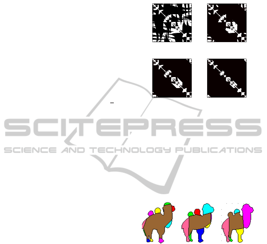
edges positioning. The G

of the camel (Figure 1(a)),

obtained by the application of the above mentioned

Visibility Rules, is depicted in Figure 1(b). As it is

obvious the structure of this matrix does not facilitate

shape partitioning. An ideal matrix for shape decom-

position would have the form of a block-diagonalsim-

ilarity matrix, where its non-overlappingblocks could

represent the shape’s parts, in a sequential manner as

it is shown in Figure 1(c). The basic idea behind this

idealization is that each shape component can be rep-

resented by a block in the respective block-diagonal

matrix

. Thus, the shape decomposition problem can

be restated as follows: Given the visibility matrix W

construct a block diagonal matrix that best approxi-

mates the desired form.

In this work we propose a technique called VSD

for solving the above deﬁned problem. In order to

achieve our goal the n-conditioned G

is introduced

and a two-step iterative algorithm is proposed for

transforming the original G

into the desired block-

diagonal form. Namely, in the ﬁrst step of the pro-

posed algorithm we attempt to “extend” the near ﬁeld

visibility by using a principle similar to the “shared

neighboors” according to which the similarity of two

nodes is conﬁrmed by the number of their Shared

Nearest Neighbors (Jarvis and Patrick, 1973). This

procedure results in a Voting graph which constitutes

the focal matrix of our decomposition scheme. In

the second stage, an appropriate thresholding proce-

dure takes place which efﬁciently converts the above

mentioned matrix into a crisp one that is used as in-

put in the next iteration of the algorithm. This itera-

tive compactiﬁcation procedure results in a block di-

agonal matrix, which best approximates the idealiza-

tion form and additionally delivers the structure of the

original shape appropriately organized into meaning-

ful groups.

Although the introduced decomposition method

does not apply the two major perception rules, i.e. the

minima rule (Singh et al., 1999b) and the short cut

rule (Singh et al., 1999a), the resulting shape cluster-

ing often corresponds well to decompositions that a

human might make. Comparisons with the state of art

methods validate that our method produces satisfac-

tory results.

The remaining of the paper is organized as fol-

lows: In Section 2 a literature overview is presented.

In Section 3 the introduced method is explained in de-

In order the ideal matrix to be block-diagonal, we

should start the decomposition from the beginning of a

group in the shape boundary. Otherwise, the ﬁrst block of

the ideal matrix is divided into four sub-blocks covering the

four corners of the matrix. However, by taking into account

their similarity and for simplicity purposes, we do not dis-

tinguish between them.

(a)

0 50 100 150 200

100

150

200

(b)

0 50 100 150 200

100

150

200

Figure 1: The camel-shape (a). The corresponding G

(b).

An ideal block diagonal matrix for the camel shape decom-

position (c). Each block in the diagonal representation de-

notes a speciﬁc shape component (d).

tail and in Section 4 experimental results are shown.

Finally the paper concludes in Section 5.

2 RELATED WORK

Shape segmentation is important in perceptual under-

standing of objects and facilitates recognition that is

robust to occlusions, movements, deletion or growth

of portions of an object (Biederman et al., 1987), (Sid-

diqi and Kimia, 1995). Shape decomposition tech-

niques, can be broadly classiﬁed into two main cate-

gories. In the ﬁrst one methods that aim to partition

a shape into its meaningful parts belong, while in the

second shapes are segmented usually by following a

certain geometric rule.

Determination of a shape part as natural is not ob-

vious due to the involvementof the human perception.

However, there exist two major rules that exploit the

results of the cognitive theory over the human’s iden-

tiﬁcation of a shape. In (Singh et al., 1999b) a set of

cuts is deﬁned, such that their endpoints denote nega-

tive minima of curvature of the corresponding bound-

ary. Continuing, in (Singh et al., 1999a) -which com-

plements the minima rule- cuts are selected according

to their length.

In (Latecki and Lak¨amper,1999) a 2D shape is de-

composed into its convex parts, at different evolution

steps, using a rule similar to minima rule. In addi-

tion, the method proposed in (Mi and DeCarlo, 2007)

is specially designed for decomposing a shape into its

meaningful parts. In (Juengling and Mitchell, 2007)

the minima and short-cut rules are used for shape de-

VISAPP2014-InternationalConferenceonComputerVisionTheoryandApplications

516

composition. In particular, a constrained Delaunay

triangulation of the shape is computed and an opti-

mum set of cuts (i.e. interior edges) is selected, by

solving a combinatorial optimization problem.

On the other hand, methods that decompose a

shape into certain geometric models usually refer to

convex parts decomposition. However, decomposi-

tion of a shape to strictly convex parts, often results in

an uncontrollablenumber of segments. Consequently,

approximate convex parts are used instead. In (Lien

and Amato, 2004) polygons are decomposed in an hi-

erarchical way, by iteratively removing the most sig-

niﬁcant non-convex parts. Authors of this paper in-

dicate the facility of computing approximate convex

segments opposed to exactly convex ones. In (Liu

et al., 2010) candidate cuts are computed by Morse

theory and their total length is minimized. In order

to avoid production of redundant parts while resulting

in natural shape decomposition, in (Ren et al., 2011)

the selection of the best set of candidate cuts that has

both a minimum size and a high visual naturalness is

proposed. The latter property is obtained by imposing

the minima rule and the short cut rule. In (Siddiqi and

Kimia, 1995) it is reported that convex parts depict in

some way the human’s conception towards decompo-

sition activities. Therefore, both (Liu et al., 2010) ,

(Ren et al., 2011) fall into both main shape decompo-

sition categories and they aim to result in meaningful

shape partitioning.

Other methods (De Goes et al., 2008) exploit the

multiscale properties of diffusion distance, in an at-

tempt to achieve robust shape decomposition in ar-

ticulated objects. In (Shapiro and Haralick, 1979) a

graph theoretic clustering method is introduced where

a 2D shape is partitioned into clusters that intuitively

correspond to shape parts. Our method is based on

a clustering technique where as we are going to see

clusters’ similarity is assessed according to an appro-

priate voting procedure.

3 THE VSD METHOD

Let us consider that the visibility matrix mentioned

in Section 1, is given. Then, the proposed method

aims at appropriately transforming the original visi-

bility matrix into a block diagonal one, which can be

easily used for the visually meaningful decomposi-

tion of the candidate shape. However, as it was al-

ready mentioned, the form of the original visibility

matrix is not appropriate to serve our goal, and must

be properly transformed. This is exactly the goal of

the following subsection.

3.1 Neighborhood Based Visibility

A shape can be easily transformed into a graph,

where the boundary points stand for the graph’s nodes

and the edges are the lines connecting those nodes.

However, such a graph has no physical signiﬁcance,

due to the fact that many nodes are connected even

though they do not “see” each other. Assuming an

observer placed at each node, a more natural re-

sult could be obtained by linking the nodes that fall

within the observer’s ﬁeld of view. According to the

Visibility Rules of Section 1, a node pair is deﬁned

as visible if its corresponding edge does not intersect

with the contour and locates inside the area enclosed

by the contour. It is clearly shown in Figure 2(a)

where nodes 1, 2 form a visible pair, while nodes 1,3

and nodes 1,4 are not visible.

(a) (b)

Figure 2: According to Visibility Rules, nodes 1,2 are vis-

ible, while nodes 1,3 and 1,4 are not visible (a). Despite

nodes i, j are visible they do not contribute to shape decom-

position as the nodes that are linked by the dotted lines (b).

Despite naturalness in the shape representation

that is introduced by the visible node pairs, there

still exist edges that do not help in distinguishing the

shape’s parts, as we can see in Figure 2(b) where the

nodes i, j form a visible pair according to the above

mentioned Visibility Rules. However, we are inter-

ested in revealing the meaningful parts of the shape,

which means that nodes i, j do not contribute to that

way as they link nodes from different shape parts. Al-

though nodes i, j can “see” each other, they are not

close neighbor points (starting from the i boundary

point and moving clock-wise). These connections

manifest themselves in Figure 3(a) as the non-zero

values that lay away from the main diagonal thus

making the solution of the shape partitioning prob-

lem complicated. On the other hand, in Figure 2(b),

nodes that are linked with i showed on dotted edges,

are found in the same neighborhood with it and form

the camel’s hump. Therefore, G

must be redeﬁned

by posing nodes’ neighborhood restriction. Speciﬁ-

cally, two boundary points are deﬁned as not visible

and their corresponding edge is set to zero, if they are

placed far from each other. Notice that distance is not

measured according to the edge length but is calcu-

lated as the number of intermediate points when mov-

AVisibilityGraphbasedShapeDecompositionTechnique

517

ing along the contour. Another interesting approach

could use edge length information, but is not studied

in this paper.

Let us concentrate ourselves on the deﬁnition of

the conditioned visibility graph. To this end, let us

deﬁne the neighborhood of radius n of the i-th node

of set V deﬁned in Equ. (2) as the following set of

indices:

= {< i+ j >

, j = 0, ±1, ±2, . . . ± n} (4)

where < . >

denotes the modulo N operation, that

is:

0 ≤ < k >

= k − mN ≤ N − 1, m ∈ Z. (5)

As it can be easily veriﬁed, the range of valid values

of radius n belongs to the set R



1, 2, ··· , ⌈

⌉



where ⌈x⌉ denotes the ceil of x. Finally, we must

stress at this point that the use of the modulo operator

is essential for the correct deﬁnition of the neighbor-

hood of a node, because the shape contours are closed

curves.

Having deﬁned the radius-n neighborhood of a

node of G

, the elements of the conditioned weighted

matrix W

can be deﬁned as follows:



, if j ∈ N

0, otherwise.

(6)

Note that the conditioned weighted matrix deﬁned

above can easily be formed from the element-wise

multiplication of the original weighted matrix W and

the following symmetric band Toeplitz matrix:

= toeplitz([1

n+1

N−(2n+1)

]) (7)

where 1

, 0

are vectors of length k containingall ones

and zeros, respectively. Note ﬁnally that the l

“norm”

of each row of the above formed matrix W

is at most

2n+ 1.

Conditioned visibility graphs resulting from the

original visibility graph of the camel shape, depicted

in Figure 3(a), are shown in Figure 3(b)-3(d) for three

(3) different values of radius n. As it is clear from this

ﬁgure, the constraint imposed through the radius of

the neighborhood of each boundary point to the ﬁeld

of view of the hypothetical observer, inﬂuences the

size, as well as, the speciﬁc form of the shape compo-

nents that emerge at a great degree. More speciﬁcally,

if the admissible number of neighboring nodes that

can be visible is small, then more yet smaller groups

of the boundary nodes have the tendency to be formed

(see Figure 3). On the other hand, imposing a loose

constraint to G

, groups have the tendency to expand,

leading, in most cases, to undesirable results. Note

also from Figure 3(a) that total absence of such a visi-

bility constraint results to a G

with non distinct com-

ponents, while edges that link nodes of physically dif-

ferent groups are present.

50 100 150 200

100

150

200

(a)

50 100 150 200

100

150

200

(b)

50 100 150 200

100

150

200

(c)

50 100 150 200

100

150

200

(d)

Figure 3: Initial G

(a) and n-conditioned G

for different

values of n: 40 (b), 30 (c) and 10 (d).

We are expecting that different values of neigh-

borhood radius, result in different decompositions of

the candidate shape. Indeed, as a rule, the greater the

radius of the neighborhood is, the larger the size of

the shape’s components are. This phenomenon, is ev-

ident in Figure 4, where the results obtained from the

application of the proposed decomposition algorithm

(presented in the next subsection) in the conditioned

visibility graphs depicted in Figure 3(b)-3(d) corre-

sponding to different values of n, are shown.

(a) n = 10 (b) n = 30 (c) n = 40

Figure 4: Different decompositions of the camel shape cor-

responding to different values of neighborhood radius n (see

text).

It is obvious that for small values of n small shape

components are constructed, but as n increases the

small components seem to merge and larger groups

are formed. As it becomes clear, we must somehow

estimate the desired radius of neighborhood of the

graph.

Moreover, although in the n-conditioned G

sev-

eral groups of boundary points seem to be formed

more clearly, as it is evident in Figure 3, a strict lim-

itation seems to be imposed by the Visibility Rules

V R

, i = 1, 2. Indeed, very often in the n-conditioned

values of boundary points are set to zero, since

according to this rule they are not visible. However,

in many cases, the majority of these nodes belong to

VISAPP2014-InternationalConferenceonComputerVisionTheoryandApplications

518

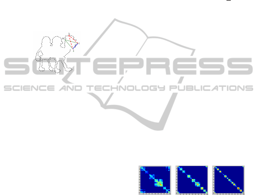
the same part of the shape. Such a case is shown,

as an example, in Figure 5 where, as it is apparent,

all nodes i, j, k and m are members of the “camel’s

head” part. Nevertheless, the boundary points i, j

cannot ”see” each other, due to the intersection exist-

ing between their corresponding edge and the shape’s

contour, which means that the i- j link gains no con-

necting value. Application of such a strict rule leaves

out many important points from each shape compo-

nent (i.e. nodes i, j in Figure 5), thus leading into

a n-conditioned G

where groups are not clearly sep-

arated and in general its form is far away from the

idealization presented in Section 1.

Figure 5: Despite violation of the rule V R

, nodes i, j are

gaining connection votes as they are both visible from nodes

k and m.

In an attempt to overcome this problem and deﬁne the

shape’s meaningful parts, as we are going to see in

the next section, we assign to each node a number that

indicates connection votes. A connection vote is as-

signed to a link each time the corresponding nodes

are both visible from another node. In Figure 5,

nodes i, j both form visible pairs with nodes k and

m, and thus two (2) votes are added to the edge ε

In that way, visibility is extended and many edges are

obtaining“visibility votes” even if they are not visi-

ble. This “indirect” visibility facilitates the connec-

tion of nodes that belong to the same group, even

though they do not all share direct links. The num-

ber of votes that an edge accumulates is analogous

to the number of nodes from which the edge’s end-

ing nodes are mutually visible. This alternative way

to deﬁne similarity between the node-pairs is similar,

but does not coincide, to the “Shared Nearest Neigh-

bors” algorithm, which was ﬁrst introduced by (Jarvis

and Patrick, 1973). According to this principle the

similarity of the connected nodes i, j which are both

connected to a set of nodes A, is augmented as their

closeness is “conﬁrmed” by nodes of set A.

Having identiﬁed the critical problems that drasti-

cally affect the quality of the solution of the problem

at hand, we are going to investigate them in detail in

the next subsection.

3.2 Neighborhood Radius Estimation

As mentioned the impact of the size of the neighbor-

hood, to the quality of the obtained shape decomposi-

tion, in terms of the visual meaningfulness of its com-

ponents, is essential. Thus its determination, even in

a non optimal way, is considered necessary. To this

end, let us consider that the idealization W

⋆

intro-

duced in Section 1, of the visibility matrix is given,

and let us form the following sequence of numbers:

c[n] =

∑

i=1

∑

j∈N

, n = 1, 2, ·· · , ⌈

⌉ (8)

where v

denotes the (i, j) element of the following

“Voting” matrix:

= W

)

= (W

)

. (9)

Note that by taking into account the special “1 − 0”

form of the components of its basic ingredient, that is

the elements of matrix W

, the content of the (i, j)-th

element of the above deﬁned voting matrix, expresses

the connectivity strength of the nodes i and j in the

shape contour. The voting matrices of the correspond-

ing n-conditioned G

shown in Figures 3(b), 3(c) and

3(d), are depicted in Figure 6, for neighborhood ra-

dius n=40, 30 and 10, respectively. Note that their

form is closer to the idealization introduced in Sec-

tion 1. This contitutes the basic reason we propose its

use as a vehicle to fulﬁll our ultimate goal, as we are

going to see in the next subsection. We have to say

more things about this voting matrix, but for the mo-

ment let us concentrate ourselves on the “Mean Vot-

ing” sequence deﬁned in Equ. (8), and in particular

on a very interesting property that it has and we are

going to exploit in order to estimate the desired value

⋆

(a) (b) (c)

Figure 6: Examples of Voting Matrices corresponding to

different values of neiborhood radius n (see text).

More precisely, using the deﬁnition of sets N

we can easily see that the cardinalities of any pair of

the aforementioned sets satisfy the following ordering

relations:

n+k

| ≥ |N

|, ∀ k ≥ 0 (10)

and consequently, as it can easily be proven, c[n] is an

increasing sequence of the neighborhood radius, that

is:

c[n+ k] ≥ c[n], ∀ k ≥ 0. (11)

In addition, there is a radius after that the values of

the sequence should not be changed even more. As it

is clear, that value is the desired n

⋆

AVisibilityGraphbasedShapeDecompositionTechnique

519

Thus, considering W

⋆

known, by computing the

sequence c[n], n = 1, 2, ··· , ⌈

⌉ from Equ. (8) and

by exploiting the above mentioned properties, the true

value of the neighborhood radius can be obtained

from the solution of the following optimization prob-

lem:

⋆

= arg max

n∈ R



c[n]

2n+ 1



. (12)

However, the ideal matrix W

⋆

is unknown and the

computation of the sequence deﬁned in Equ. (8) is

practically impossible. Instead, the use of the ac-

tual n-conditioned visibility matrices is proposed for

its evaluation and then an estimation of the desired

neighborhood radius ˆn

⋆

can be achieved by solving

the corresponding optimization problem. An example

of the above mentioned sequences resulting from the

solution of the above mentioned optimization prob-

lems to the “octapus” shape is shown in Figure 7. We

must stress at this point that even though the exact

and the approximated sequences are totally different,

the values of the corresponding neighborhoodradii, in

most cases, are close to each other. Furthermore, the

impacts of “dark areas” along the main diagonal as

well as the off diagonal “bright areas” appeared in the

sequence of the actual matrices are clearly depicted

on the form of “Mean Voting Actual” sequence shown

in Figure 7(d).

(a)

20 40 60 80 100 120 140 160 180 200

100

120

140

160

180

200

(b)

20 40 60 80 100 120 140 160 180 200

100

120

140

160

180

200

(c)

0 10 20 30 40 50 60 70 80 90 100

500

1000

1500

2000

2500

3000

Neighborhood Radius n

Mean Voting Sequences

Ideal

Actual

(d)

Figure 7: The octapus shape contained in MPEG7 CE-

shape1 part B (a), its ideal block diagonal matrix (b), the

actual ˆn

⋆

-conditioned G

Voting” sequences (d).

Having estimated the neighborhood radius ˆn

⋆

for

a candidate shape, let us go back to “Voting” matrix

deﬁned in Equ. (9) and see how we can use it to

solve the second critical problem mentionedin the last

paragraph of the previous subsection.

3.3 The Iterative Algorithm

What remains in order to complete the presentation

of the proposed technique is the development of an

algorithm for the solution of the inverse problem, that

is, given the actual conditioned visibility matrix W

⋆

form a block diagonal matrix with each block repre-

senting a meaningful part of the shape contour. To

this end, we propose a two step iterative algorithm

with its ﬁrst step being a normalization-step of the

“Voting” matrix V

deﬁned in Equ. (9) and the sec-

ond one a thresholding-step. Let us now concentrate

on the above mentioned matrix and see how we can

use it in order to achieve our goal. As it is clear from

its deﬁnition in Equ. (9), the (i, j) element of the ma-

trix can be expressed by the inner product of the i-th

and j-th rows of the matrix W

⋆

, that is:

⋆

=< w

⋆

, w

⋆

> . (13)

Using the deﬁnition of the inner product, Equ. (13)

can be rewritten as follows:

⋆

= ||w

⋆

||w

⋆

cos(θ

) (14)

where ||x||

denotes the l

norm of visibility vector x,

and θ

the existing angle between the two mentioned

visibility vectors.

We can now deﬁne the following normalized ver-

sion of the above mentioned matrix

¯v

⋆

= cos(θ

) (15)

with the value of each element, quantifying the exist-

ing similarity or correlation of the visibility vectors

corresponding to nodes i and j of the

⋆

-conditioned

visibility graph.

Note now that after the normalization step, matrix

⋆

takes values in the interval [0 1], and thus our

goal now is to update the W

⋆

by using a predeﬁned

threshold t:

⋆

≥ t (16)

and use it as the new approximation of the ideal visi-

bility matrix in the next iteration.

The above described steps are repeated in an itera-

tive fashion until the convergence to a block diagonal

matrix be achieved.

An outline of the proposed algorithm follows.

procedure SHAPE DECOMPOSITION(V , t)

Using V R

, i = 1, 2, form matrix W

Form c[n], n = 1, 2, · ·· , ⌈

⌉ of Equ. (8).

Solve Problem deﬁned in (12) to ﬁnd ˆn

⋆

Form W

ˆn

⋆

using W and T

ˆn

⋆

of Equ. (7).

repeat

Form the Normalized Voting matrix

ˆn

⋆

VISAPP2014-InternationalConferenceonComputerVisionTheoryandApplications

520

using Equ. (15).

Use Equ. (16) to update matrix W

ˆn

⋆

until convergency

end procedure

Having completed the presentation of the pro-

posed technique, in the next section we are going

to apply it on several shapes and compare its perfor-

mance against well knownin the literature techniques.

4 EXPERIMENTAL RESULTS

In this section we are going to present comparative

results obtained from the application of the proposed

technique on several shapes of the MPEG7 CE-shape-

1 part B database (Latecki et al., 2000). All shape

contours we used in our experiments, were sampled

at N=200 points. In addition, in all experiments we

have conducted, the value of threshold t was set to

0.5.

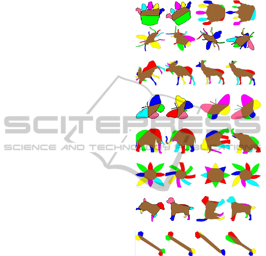
A sample of 2D decomposed shapes are shown in

Figure 8. It is evident that for some shapes the re-

sulting decomposition is meaningful, while in some

situations, parts that obviously could not be sepa-

rated by a human being, are splitted by the algorithm.

Speciﬁcally, the crown shapes are decomposed into

seven (7) or eight (8) parts, while one could expect

a six-part result. Continuing, in the ﬂy shapes legs,

wings and antennas are successfully recognized by

our method. The same comment holds for the but-

terﬂies shown in the fourth row of the ﬁgure. More-

over, in shapes such as the deer, the elephants and

the dogs, the introduced method achieves partition-

ing into meaningful components (i.e. legs, head, tails

etc). However, in some cases the start and the end

boundary points of a component should be deﬁned

more explicitly, so as to better demostrate the mean-

ingful component that is captured. Finally, shapes

such as the bone or the margaret-like ones, are well

partiotioned. Regarding the non-rigid parts of shapes

(i.e. legs, tails, proboscis, antennas etc) we can ob-

serve that the VSD method provides satisfactory re-

sults, as it achieves to recognize almost all meaning-

ful articulated shape parts, even if they are depicted in

different poses. Despite the fact that non-rigid defor-

mations affect the visibility graph (different edges are

revealed, while others may dissapear), the key idea of

connection votes, seems to give the ability to handle

non-rigid shape variations, in an effective way.

To further demonstrate the effectiveness of the

proposed technique, a small sample of the results we

obtained from the application of our technique as well

as the ACD (Lien and Amato, 2004), the CSD (Liu

Figure 8: A sample of decomposed shapes of the MPEG7

database.

et al., 2010) and the MNCD (Ren et al., 2011) meth-

ods on shapes contained in the MPEG7 CE-shape-1

part B database, are shown in Figure 9. As we can

see from this ﬁgure, the proposed method performs

well in cases of non-rigid parts. Indeed, the beetle’s

legs as well as the horse’s legs are not decomposed

into multiple parts, an indication that the results of the

proposed technique are close to perceptually mean-

ingful decompositions. On the other hand, methods

that use concavity rules fail to capture such parts as

a whole, because of their large concavity. Having

no intention to discredit the performance of the other

techniques, the VSD fails to recognize the head of the

AVisibilityGraphbasedShapeDecompositionTechnique

521

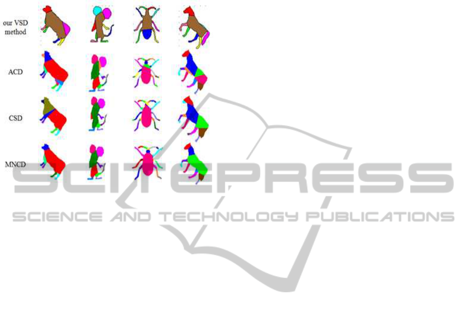
mouse shape as a whole part due to the constraint that

is imposed to the Visibility Graph by the estimated

value ˆn

⋆

of radius.

Figure 9: A small sample of decomposition results obtained

from the application of our method and ACD, CSD and

MNCD methods in shapes contained in MPEG7 database.

5 CONCLUSIONS

In this paper, a novel method for shape decomposi-

tion is presented, which stems from the idea of vis-

ibility between boundary points. The shape is seg-

mented into its meaningful parts by a two-step al-

gorithm which efﬁciently organizes shape’s boundary

points into separate blocks. The proposed method is

applied in a large number of 2D shapes. The intro-

duced technique seems to result in perceptualy more

meaningful decompositions of the non-rigid parts of

the shapes, than most of the existing methods. In ad-

dition, the proposed technique results in decomposi-

tions that nearly captures the whole structure of the

original shape. The extension of the proposed tech-

nique in 3D shapes and the development of new ro-

bust algorithms to efﬁciently convergeto the ideal low

rank shape matrix are currently under investigation.

REFERENCES

Biederman, I. et al. (1987). Recognition-by-components: A

theory of human image understanding. Psychological

review, 94(2):115–147.

De Berg, M., Van Kreveld, M., Overmars, M., and

Schwarzkopf, O. (1997). Computational geometry:

algorithms and applications. Springer.

De Goes, F., Goldenstein, S., and Velho, L. (2008). A hier-

archical segmentation of articulated bodies. In Com-

puter graphics forum, volume 27, pages 1349–1356.

Wiley Online Library.

Jarvis, R. and Patrick, E. (1973). Clustering using a similar-

ity measure based on shared nearest neighbors. Pat-

tern Analysis and Machine Intelligence, IEEE Trans-

actions on, 22(11).

Juengling, R. and Mitchell, M. (2007). Combinatorial shape

decomposition. In Advances in Visual Computing,

pages 183–192. Springer.

Latecki, L. J. and Lak¨amper, R. (1999). Convexity rule for

shape decomposition based on discrete contour evo-

lution. Computer Vision and Image Understanding,

73(3):441–454.

Latecki, L. J., Lakamper, R., and Eckhardt, T. (2000). Shape

descriptors for non-rigid shapes with a single closed

contour. In Computer Vision and Pattern Recognition,

2000. Proceedings. IEEE Conference on, volume 1,

pages 424–429. IEEE.

Lien, J.-M. and Amato, N. M. (2004). Approximate convex

decomposition of polygons. pages 17–26.

Liu, H., Liu, W., and Latecki, L. J. (2010). Convex

shape decomposition. In Computer Vision and Pat-

tern Recognition (CVPR), 2010 IEEE Conference on,

pages 97–104. IEEE.

Liu, Y.-S., Ramani, K., and Liu, M. (2011). Computing

the inner distances of volumetric models for articu-

lated shape description with a visibility graph. Pat-

tern Analysis and Machine Intelligence, IEEE Trans-

actions on, 33(12):2538–2544.

Mi, X. and DeCarlo, D. (2007). Separating parts from 2d

shapes using relatability. In Computer Vision, 2007.

ICCV 2007. IEEE 11th International Conference on,

pages 1–8. IEEE.

Ren, Z., Yuan, J., Li, C., and Liu, W. (2011). Minimum

near-convex decomposition for robust shape represen-

tation. In Computer Vision (ICCV), 2011 IEEE Inter-

national Conference on, pages 303–310. IEEE.

Shapiro, L. G. and Haralick, R. M. (1979). Decomposition

of two-dimensional shapes by graph-theoretic cluster-

ing. Pattern Analysis and Machine Intelligence, IEEE

Transactions on, (1):10–20.

Siddiqi, K. and Kimia, B. B. (1995). Parts of visual form:

Computational aspects. Pattern Analysis and Machine

Intelligence, IEEE Transactions on, 17(3):239–251.

Singh, M., Seyranian, G., and D.Hoffman (1999a). Parsing

silhouettes: The short-cut rule. Perception and Psy-

chophysics, 61(4):636–660.

Singh, M., Seyranian, G. D., and Hoffman, D. D. (1999b).

Parsing silhouettes: The short-cut rule. Perception &

Psychophysics, 61(4):636–660.

VISAPP2014-InternationalConferenceonComputerVisionTheoryandApplications

522