Non-rigid Registration for Deformable Objects

Van-Toan Cao, Van Tung Nguyen, Trung-Thien Tran, Sarah Ali and Denis Laurendeau

Computer Vision and Systems Laboratory, Department of Electrical and Computer Engineering, Laval University,

1065 Avenue de la M

edecine, G1V 0A6, Qu

ebec, Canada

Keywords:

Registration, Deformation, Correspondences, Optimization.

Abstract:

We present an efﬁcient algorithm for non-rigid registration of two partially overlapping 3D surfaces in which

a target surface is a deformed instance of a source surface. The algorithm is implemented in two main phases.

In the ﬁrst phase, the robust algorithm that is used is based on a probability density estimation to ﬁnd reliable

correspondences between the two surfaces. Then, in the second phase, a deformation algorithm is applied

for non-rigid registration where the displacement of each point is described by an afﬁne transformation in

relation with other points of the same surface and its corresponding point on the other surface. Combined with

initial correspondences in the ﬁrst phase, an effective strategy for optimization of a cost function is carried out

to align the two surfaces without using any assumption and user-intervention on the algorithm. We test the

robustness of our method by efﬁciently aligning pairs of surfaces of realistic scan data of human body models.

1 INTRODUCTION

Registration of two surfaces is a well-known problem

and a key task in computer graphics where two sur-

faces are partial digital representations of the same

object but are taken at different times or/and differ-

ent locations. To align such surfaces into a common

coordinate system, parameters must be computed for

the movement of the source surface onto the target

surface. For cases where the object is a rigid body,

the problem of general registration reduces to a rigid

registration problem and the movement between two

surfaces is described globally by a rotation matrix, a

translation vector (or/and a scaling coefﬁcient). Many

algorithms have been proposed to address rigid regis-

tration and it is now considered to be almost solved.

Thus attention is shifting to dealing with non-rigid

registration where the object undergoes deformations

when being scanned and the movement between two

surfaces cannot be described by a single rigid trans-

formation.

Many algorithms are proposed to ﬁnd the move-

ment in a non-rigid registration paradigm with differ-

ent strategies and assumptions. A common strategy

of many of these algorithms is to associate a transfor-

mation for each respective point on the source surface

and move each point to a corresponding point on the

target surface while imposing coherence constraints

with other points. For this step, the optimization of

these methods uses some assumptions to obtain the

ﬁnal alignment.

In this paper, we present an algorithm to align two

partially overlapping surfaces (in our case, they are

two meshes but the framework of the algorithm can be

applied to other surface representations) for address-

ing the challenges of non-rigid registration. Gener-

ally, each point of the source surface will have its own

transformation to move it correctly to its correspond-

ing point on the target surface. To achieve that, the

optimization of the cost function requires that stable

correspondences be found and the correct transforma-

tions to align two surfaces be estimated. Since con-

vergence to a wrong minimum of the cost function is

not desired, some methods put user-deﬁned makers

on the two surfaces to guide the optimization process.

Other approaches assume the movement between the

two surfaces is small, or that poses of the two sur-

faces are the same. However, our algorithm does not

use any assumption for the optimization and automat-

ically performs without any user-intervention. The al-

gorithm is implemented in two phases. In the ﬁrst

phase, a robust method based on probability density

estimation provides a set of candidates as correspon-

dences between the two surfaces. In the second phase,

these candidates are used as initial correspondences

and combined with an effective optimization strategy

to guide the algorithm to converge to a minimum.

Cao V., Nguyen V., Tran T., Ali S. and Laurendeau D..

Non-rigid Registration for Deformable Objects.

DOI: 10.5220/0004683100430052

In Proceedings of the 9th International Conference on Computer Graphics Theory and Applications (GRAPP-2014), pages 43-52

ISBN: 978-989-758-002-4

 2014 SCITEPRESS (Science and Technology Publications, Lda.)

2 RELATED WORK

The goal of registration algorithms is to align two

surfaces together to obtain a better representation of

the object. If the object is rigid, one global transfor-

mation is sufﬁcient to describe the movement of the

source surface and to align it to the target surfaces.

The Iterative Closest Point algorithm (ICP)(Besl and

McKay, 1992; Chen and Medioni, 1991) and its vari-

ants (Rusinkiewicz and Levoy, 2001) are prominent

among rigid registration algorithms due to their sim-

plicity and robustness. ICP iteratively searches for

correspondences based on a closest distance criterion

for ﬁnding a rigid transformation until it reaches a lo-

cal minimum. A limitation of ICP is that it is only

effective when a good initial registration between the

two surfaces is available or when the movement be-

tween the two surfaces is small.

Based on the ICP, a variety of techniques have

been adapted to the problem of non-rigid registration

(Brown and Rusinkiewicz, 2007; Allen et al., 2003;

Amberg et al., 2007; Pauly et al., 2005; Huang et al.,

2008). However, like ICP, these algorithms need to

use prior knowledge to avoid converging to a wrong

local minimum of the cost function. In (Allen et al.,

2003; Amberg et al., 2007; Allen et al., 2002) a tem-

plate model, which is the same pose as the scanned

surface, provides a strong geometric prior for recon-

structing high-quality models with automated hole-

ﬁlling and noise removal. Moreover, user-deﬁned

markers placed on the template model and scanned

surface are exploited to prevent the optimization al-

gorithm to set stuck in a local minimum.

Some algorithms are proposed to take advantage

of real-time 3D scanners. They do not use any tem-

plate or user-deﬁned markers for alignment. In (Mi-

tra et al., 2007; Submuth et al., 2008), registration

is conducted without computing correspondences ex-

plicitly. These algorithms aggregate all scans into a

4D space-time surface and estimate inter-frame mo-

tion from kinematic properties of this surface. In

(Wand et al., 2009), a hierarchical registration ap-

proach is applied where the algorithm aligns every

two frames, merges them, then aligns every two pairs

of frames, merges them, and so on until it processes

the entire sequence. These algorithms fail when the

input data is noisy and the deformation between two

surfaces is large.

Recent algorithms attempt to remove the depen-

dency on template models or artiﬁcial markers. In

(Huang et al., 2008), a set of geodesically consis-

tent correspondences are extracted and the algorithm

solves for transformations at many sampled locations

on the surface and then interpolates the remaining

surfaces using prescribed inﬂuence weights. This

method can solve for large deformation where the as-

sumption of geodesic consistency between two sur-

faces is warranted. Chang et al. (Chang and Zwicker,

2008) determine the correspondences by spin image

(Johnson, 1997) and ﬁnd transformation for each pair

of matches. Based on non-linear mean-shift frame-

work, they then cluster transformations between two

surfaces into many groups before applying a graph-

cut technique to associate each transformation for

each point on the two surfaces.With this algorithm,

some transformations do not exist in the motion sam-

pling process, this causes some parts on the source

surface to lack a precise transformation to align cor-

rectly with the respective parts on the target surface.

Li et al. (Li et al., 2008) applied an embedded defor-

mation algorithm to solve for a reduced set of trans-

formations. During optimization of the cost function,

their algorithm exploits a 2D parameterization of the

range scans to search for closest points on the target

scan as corresponding points and guide the optimiza-

tion to converge to a local minimum. Therefore, their

algorithm is limited to 3D scans. Moreover, if the

movement between two scans is large, this algorithm

can be trapped in a wrong local minimum. Our algo-

rithm does not need a parameterization of the range

scan and can deal with other surface representations.

Moreover, we use initial correspondences as an opti-

mization constraint to achieve a correct alignment for

large deformations.

In (Anguelov et al., 2004), the method ﬁnds a

good correspondence assignment with a given tem-

plate shape by formulating a Markov Random Field

optimization that best ﬁts the observed data and pre-

serves the shape of the template. The method is able

to recover signiﬁcant movements of articulated parts

and non-rigid deformation. This method assumes that

preservation of geodesic distance is warranted and

one of the input shapes is a subset of the others. My-

ronenko et al. (Myronenko and Song, 2010) con-

sider the alignment of two point sets as a probabil-

ity density estimation problem. Their algorithm ﬁts

Gaussian Mixture Model (GMM) centroids (source

point set) to the data (target point set) by maximiz-

ing the likelihood. The GMM centroids are moved

coherently as a group to preserve topological struc-

ture of the point sets. Experimental results show that

this method outperforms another well-known method

(Chui and Rangarajan, 2003). In a similar work, al-

gorithm of Jian et al. (Jian and Vemuri, 2011) mini-

mizes a statistical discrepancy measure between two

mixture models in which each model is a Gaussian

mixture model and presents an input point set. How-

ever, a bottleneck of these three methods is that they

GRAPP2014-InternationalConferenceonComputerGraphicsTheoryandApplications

require signiﬁcant computation as well as large mem-

ory space to describe the relationship between each

point of the ﬁrst point set and each point of the second

point set at each iteration of the optimization process

(for more detail, we refer the reader to (Myronenko

and Song, 2010)). Therefore, this approach is mostly

applied to 2D data or small 3D data sets.

3 PROPOSED METHOD

3.1 Deformation Model

Because we need to move each point on the source

surface to its corresponding point on the target sur-

face, computation becomes too cumbersome to search

for a transformation for each point of the source sur-

face. A deformation model is necessary to reduce

the computation time. The chosen model also has

to be general enough to apply to any object and ex-

press complex deformations. Given these goals, we

adopted the deformation model proposed by Sumner

et al. (Sumner et al., 2007) for our algorithm. For

this model, a space deformation is deﬁned by a col-

lection of afﬁne transformations. The graph of the

model consists of nodes and undirected edges. While

nodes are chosen by uniformly sampling the source

surface and one transformation is associated to each

node, undirected edges connect nodes of overlapping

inﬂuence to indicate local dependencies. Given the

node position g

∈ R

, j ∈ 1 ...m , the afﬁne transfor-

mation for this node is speciﬁed by a 3x3 matrix R

and a 3x1 translation vector t

. The inﬂuence of the

transformation is centered at the node’s position so

that it maps any point p in R

to position

p according

to:

p = R

(p − g

) + g

+ t

(1)

The inﬂuence of individual nodes is smoothly

blended so that the deformed position

of each point

on the source surface v

is a weighted sum of its posi-

tion after application of the deformation graph afﬁne

transformations.

∑

j=1

)



− g

) + g

+ t



(2)

The weights for each point are precomputed ac-

cording to:

) = (1 − kv

− g

k/d

max

)

(3)

and then normalized to sum to one. Here, d

max

is the

distance to the k + 1 nearest node. Once the deforma-

tion graph has been speciﬁed, the optimization will

treat per-node afﬁne transformations as unknowns for

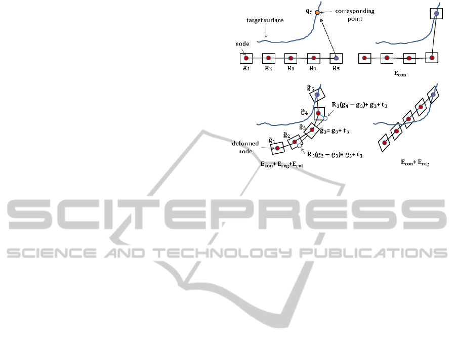
Figure 1: Effect of the three energy terms in a simple de-

formation graph. The quadrilaterals at each node illustrate

the deformation induced by the respective afﬁne transfor-

mation.

deformation. Constraints are needed so that the defor-

mation is natural and preserves topology of the source

surface. The ﬁrst energy term, E

rot

, penalizes devia-

tion of each transformation from a pure rigid motion:

rot

∑

j=1

Rot(R

) (4)

where

Rot(R) =(c

· c

)

+ (c

· c

)

+ (c

· c

)

· c

− 1)

+ (c

· c

− 1)

+ (c

· c

− 1)

(5)

and c

, c

and c

are column vectors of R

The second energy term, E

reg

, serves as a regular-

izer for the deformation by indicating that the afﬁne

transformations of adjacent graph nodes should agree

with one another:

reg

∑

j=1

∑

k∈N ( j)

−g

)+g

−(g

)

(6)

where N ( j) is a set of neighbor nodes of node j.

The third energy term, E

con

, penalizes the devi-

ation of each deformed node and its corresponding

point:

con

∑

j=1

− q

(7)

Here,

is deformed position of node j. A description

for deformation model (Sumner et al., 2007) is shown

in Figure. 1.

In our case, q

is the corresponding point of g

not deﬁned by the user. In the best case, we hope

that each node has its corresponding point to guide

Non-rigidRegistrationforDeformableObjects

the deformation leading to the target surface perfectly.

However, due to partial overlap between the two sur-

faces, some nodes on the source surface will not have

a corresponding point on the target surface.

Let’s deﬁne a cost function:

E = w

rot

+ w

reg

+ w

con

(8)

where w

rot

reg

con

refer to the contribution weight

of each energy term.

Given m nodes in the deformation graph, the op-

timization for the cost function E has to ﬁnd optimal

values of 15m unknowns. Here, each node has 12 un-

knowns for its associated afﬁne transformation and 3

unknowns for the 3D coordinates of its correspond-

ing point. All unknowns are stacked into a column

vector z and the optimal value of z will be obtained

by our strategy when combined with the Levenberg-

Marquardt algorithm (Madsen et al., 2004). The opti-

mization is separated into two steps, called movement

optimization and alignment optimization.

3.2 Finding Reliable Correspondences

A corresponding point q

must be determined for

each node to apply Eq. 7 to start the optimization

problem (Eq. 8). Since we do not exploit user-deﬁned

markers, an automatic method is thus desired to ob-

tain correspondences. For rigid registration, 3D shape

descriptors (Johnson, 1997; Frome et al., 2004; Mian

et al., 2004) can provide correspondences. However,

it becomes difﬁcult to apply these descriptors for non-

rigid registration because changes between the two

surfaces are not only due to a global movement but

also to local deformations such as bulging, stretching,

bending or ﬂapping.

Instead of using geometry-based descriptors to

ﬁnd correspondences, we use a probability-based

method for this purpose. The Coherent Point Drift

(CPD) algorithm proposed by Myronenko et al. (My-

ronenko and Song, 2010) satisﬁes this requirement.

Their algorithm uses a probability approach to align

two point sets robustly. Moreover, it also provides

the correspondences between the two point sets. The

algorithm deﬁnes the correspondence probability be-

tween a point y

(centroid) on the source point set

and a point x

(data point) on the target point set as

the posterior probability of the GMM centroid given

the data point p(y

| x

) = p(y

)p(x

| y

)/p(x

). Be-

cause the number of points between the two sets are

different, we cannot achieve one-to-one correspon-

dences and thus one point in the source set can have

more than one corresponding point in the target set.

Given nodes of the deformation graph, we need to

inspect which points are actual correspondences for

these nodes.

As mentioned above, the CPD approach is not ef-

ﬁcient when applied to large data sets due to its com-

putation burden. So, given the data in the source sur-

face V, uniform sampling is used to reduce the size of

the data. Then, the reduced data set is concatenated

with the data of the deformation graph G to create an-

other source data set Y. This process is also applied

to the target surface Q to create another target data set

X. Then, the correspondences between the new data

sets Y, X are computed with the CPD. Two additional

steps are used for evaluation of the correspondences.

First, for each pair of correspondences, the Eu-

clidean distance between deformed point

and its

corresponding point x

is computed. These distances

are then used to build a distance distribution. In this

distribution, there are two cases for which some dis-

tance values differ signiﬁcantly. In the ﬁrst case, be-

cause the CPD can give incorrect alignment of some

patches between the two data sets, some correspon-

dences belonging to these patches will be erroneous

and thus result in large distances. In the second

case, because the two data sets overlap partially, some

patches of the source data do not exist on the target

data, and vice-versa. However, the CPD always pro-

vides a corresponding point for each point on these

patches; the correspondences are also erroneous and

result in large distances. In both cases, these large

distances are treated as outliers in the distance distri-

bution. To detect these outliers, a standard statistical

procedure is to determine the “fourth spread” of the

distance distribution (DeVore, 2008).

= m

− m

(9)

where m

is median of largest L/2 measurements, m

is median of smallest L/2 measurements, L is number

of distance values.

Statistically moderate outliers are 1.5 f

units

above (below) the upper (lower) fourth, and extreme

outliers are 3 f

units above (below) the upper (lower)

fourth. In our experiment, we choose the moderate

threshold T

= 1.5 f

+ m

to detect outliers. Given

threshold T

, the corresponding point to each node

will be removed if the distance is larger than this

threshold.

In the second step of the correspondence evalua-

tion, we check if the corresponding points of the re-

maining nodes are reliable or not. At this point, a

spin image-based method (Johnson, 1997) is used.

The spin-image is not robust enough to ﬁnd corre-

spondences, especially for deformable objects, when

each spin image of a point on the source surface is

compared with all spin images of points on the tar-

get surface. There are many similar spin images of

the points on the target surface, thus this comparison

yields many erroneous correspondences. However,

GRAPP2014-InternationalConferenceonComputerGraphicsTheoryandApplications

in our case, the corresponding points of nodes in the

graph are known by the CPD and spin images become

useful for checking whether these correspondences

are sufﬁcient or should be removed. So, given two

spin images I

and I

of a node and its corresponding

point (Note that during spin image computation for

each node and its corresponding point, the points on

the original surfaces V, Q are used), we measure the

similarity between these two images using Eq. 10:

C(I

) = [atanh(R(I

))]

− λ



M − 3



(10)

where

R(I

) =

∑

−

∑

− (

∑

)

][M

∑

− (

∑

)

]

(11)

is a linear correlation coefﬁcient; u

are spin image

values at pixels; M is number of overlaping pixels be-

tween two spin images; and λ weighs the importance

of the correlation coefﬁcient against the conﬁdence in

this coefﬁcient.

With a predeﬁned threshold T

, the remaining

nodes will have reliable corresponding points if sim-

ilarity measures Cs between these nodes and respec-

tive corresponding points are greater than T

3.3 Optimization

3.3.1 Movement Optimization

We set w

rot

= 1000,w

reg

= 100 and w

con

= 10. It

means that rigid movement and regularization con-

straints are favored at the beginning of the optimiza-

tion while the position constraint is kept small but

guarantees that the deformation graph does not drift

far away from the target surface. This setup en-

sures strong stiffness for the deformation and thus the

nodes do not move directly towards their correspond-

ing points, but move parallel to the target surface.

We now need to determine how the optimization

identiﬁes the corresponding points. To do this, we di-

vide the nodes of the deformation graph into two sub-

sets. The ﬁrst subset, G

cor

, consists of nodes whose

reliable corresponding points are obtained according

to the procedure described in the previous section

(phase 1). The second subset, G

clo

, consists of nodes

which do not have corresponding points before the

optimization. For the nodes in G

cor

, we do not want

their corresponding points to be ﬁxed during the opti-

mization, but rather give the chance for each node to

ﬁnd a new one surrounding its corresponding point.

The deformation graph is thus more ﬂexible when it

approaches the target surface and it is still warranted

Figure 2: Based on reliable correspondences and an effec-

tive strategy for the optimization, our algorithm ﬁnds cor-

rect alignment between two deformable surfaces.

to follow the right direction. Therefore, at each corre-

sponding point on the target surface, we deﬁne a ra-

dius r to create a region in which the node can search

for a closest point as a new corresponding point at

the current iteration (Figure. 2). For remaining nodes

in G

clo

, their corresponding points are identiﬁed by a

closest point method on the entire target surface based

on a kd-tree algorithm.

While the E

rot

and E

reg

terms prevent the topology

of the deformation graph from being destroyed during

the optimization, the E

con

term plays an essential role

in pulling the source surface toward the target sur-

face. If we deﬁne group A consisting of the nodes in

cor

and their respective corresponding points; group

B consisting of the nodes in G

clo

and their respec-

tive corresponding points, then elements in group A

have stronger conﬁdence than those in group B for

this movement. Consequently, we want the contribu-

tion of group A to E

con

to be greater than that of group

For this purpose, for group A, the contribution of

each correspondence is weighed by w

con

and w

con

. For group B, we ﬁrst compute the Euclidean

distances of the correspondences to make a distance

distribution and the median value m

of this distri-

bution is computed. Then, the contribution of each

correspondence of the ﬁrst half of the correspon-

dences whose Euclidean distances are less than m

weighed by w

con

= w

con

= w

con

. However, the contri-

bution of the second half of correspondences whose

Euclidean distances are greater than m

is different.

Let D

be the total distance of the second half

of correspondences, and d

be the distance of each

correspondence of this half. Then, the contribution of

each correspondence to the E

con

term is calculated by:

con

= (1 −

con

(12)

The weight w

con

indicates that, for correspon-

dences of the second half obtained by the closest point

method, the greater the distance, the less useful the

Non-rigidRegistrationforDeformableObjects

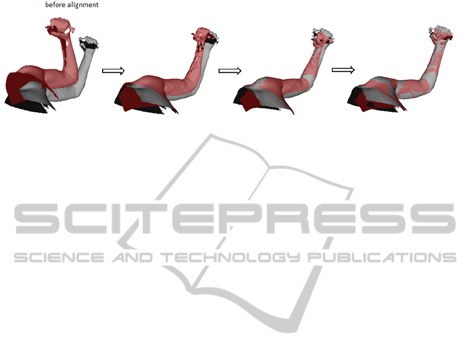
Figure 3: Alignment at different cycles in movement optimization.

correspondences are in the cost function during move-

ment optimization.

After determining the various contributions to the

cost function E, the optimization is started. When

the deformation graph is far away from the target sur-

face, the prominent weights for the rigid energy term

and the regularization energy term make the nodes

of the deformation graph move parallel to the target

surface. After that, we want to reduce the importan-

nce of these terms when the deformation graph ap-

proaches the target surface. To achieve this, an au-

tomatic method is employed to update the weights.

First, the optimization process runs with a weight set

rot

reg

con

) = (1000,100, 10) until the cost func-

tion meets one of two following convergent critera at

iteration l:

− E

l−1

< 10

−4

− z

l−1

< 10

−6

(13)

Then, this optimization process restarts a new cy-

cle in which w

rot

and w

reg

are reduced by half while

con

remains constant. This stratergy is repeated un-

til the w

rot

< 5 and w

reg

< 0.5. This whole process is

called movement optimization. A sequence of align-

ments at different cycles of the movement optimiza-

tion is shown in Figure. 3.

3.3.2 Alignment Optimization

When the movement optimization is completed, it

provides a value z

which pulls the deformation graph

close to the target surface. However, z

is not an op-

timal value when the deformation graph cannot align

correctly with the target surface. Consequently, it is

necessary to improve this value of z

to achieve con-

vergence toward minimum of the cost function E. An

alignment optimization is thus carried out.

For the alignment optimization, the corresponding

points of nodes in G

cor

and G

clo

are redeﬁned. In this

optimization, we do not distinguish whether a corre-

sponding point is found by using solely the closest

point computation or being based on the node’s reli-

able corresponding point in the ﬁrst phase. All cor-

responding points of the nodes are found by the clos-

est point method. Because convergence of the cost

function can be inﬂuented by poor correspondences,

two tests are used to dectect these correspondences.

In the ﬁrst test, a contribution of a correspondence

to E

con

will be ignored if the corresponding point of

the respective node is located on the boundary of the

target surface. In the second test, the contribution

is removed if the angle between the normal of the

corresponding point and the normal of the respective

deformed node is greater than a ﬁxed threshold T

where the normal of a point is transformed by:

∑

j=1

−1T

(14)

The weights for E

rot

reg

and E

con

and other ini-

tial values in the alignment optimization are inherited

from the ones at the last iteration of the ﬁnal cycle of

the movement optimization. We obtain the optimal

value z

∗

if one of two following criteria is satisﬁed:

− E

l−1

< 10

−7

− z

l−1

< 10

−7

(15)

Once the afﬁne transformations are found by opti-

mization, the deformation of each point on the source

surface is computed using Eq. 2. Due to the graph

structure, transformations that are close to one an-

other will be the most similar. Thus, for consistency

and efﬁciency, we limit the inﬂuence of the deforma-

tion graph on a particular point to the k-nearest nodes.

In our experiment, we use k = 4 or k = 8.

4 RESULTS

In this section, we evaluate our algorithm with real

data sets which consist of meshes built from scanned

parts of the human body. These data sets present

GRAPP2014-InternationalConferenceonComputerGraphicsTheoryandApplications

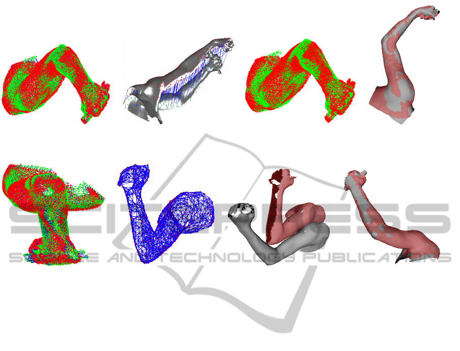
(a) CPD result (b) Correspondences (c) Alignment for reduced original data (d) Result of our algorithm

Figure 4: Non-rigid registration for two surfaces where the deformation between two surfaces is large.

(a) CPD result (b) Deformation graph (c) Before alignment (d) Result of our algorithm

Figure 5: Our result for non-rigid registration although the CPD provides misalignment.

scanned objects which undergo a large deformation

between the two scans.

In Figure. 4, we show the steps of our method ap-

plied to real data representing a human arm at two

different poses. The number of data points on the

original source surface V

and target surface Q

are

= 49427 and N

= 47735 respectively. Af-

ter reducing the original data and creating a defor-

mation graph, the number of points in the two point

sets Y

and X

are N

= 8504 and N

= 7978

respectively where the number of nodes in Y

= 536. The two surfaces are very far away from

each other, deformation between them is large, and

data in the hand area of the source surface is missing

on the target surface. Without prior knowledge, the

optimization implemented by many algorithms (Allen

et al., 2003; Amberg et al., 2007; Mitra et al., 2007;

Chang and Zwicker, 2008; Li et al., 2008) will pro-

vide a non-optimal value and result in poor align-

ment. However, using the CPD (Figure. 4(a)) com-

bined with phase 1 of our method, reliable correspon-

dences (Figure. 4(b)) are obtained. These correspon-

dences initialize the optimization process and guide

the algorithm toward a good alignment (Figure. 4(d)).

Figure. 4(c) shows our result for reduced data. When

compared with the alignment achieved by CPD, align-

ment results are almost similar between the two meth-

ods. However, while the CPD is used for the reduced

data set, our method can be applied to the original

data (large data) set based on the deformation model

(Eq. 2).

The next experiment is performed on two surfaces

of the arm with the number of data points (N

, N

, m

) = (40905,47534,8703,7987,629).

A question that is considered is whether or not the

deformation result of the CPD on reduced data can

be used to continue the optimization on the original

data. This means that we can sample the deformed

data in the CPD result uniformly to create a defor-

mation graph. Then, the optimization for the original

data is initiated with this deformation graph.

This approach can help to accelerate the optimiza-

tion. However, in our experiment, we are aware of

a potential danger because this procedure can de-

stroy the ﬁnal alignment of original surfaces if the

deformed data of the CPD result does not align well

with the reduced target data. Consequently, the defor-

mation for the original data is executed on a wrong

deformation graph. In Figure. 5(a), the CPD provides

an incorrect alignment where the deformed reduced

data (red data) is not ﬁtted well with the reduced tar-

get data (green data) near the wrist. Therefore, we al-

ways create the deformation graph from the original

source surface (Figure. 5(b)). Our result for this ex-

periment is shown in Figure. 5(d) where the alignment

near the wrist is correct although there is missing data

Non-rigidRegistrationforDeformableObjects

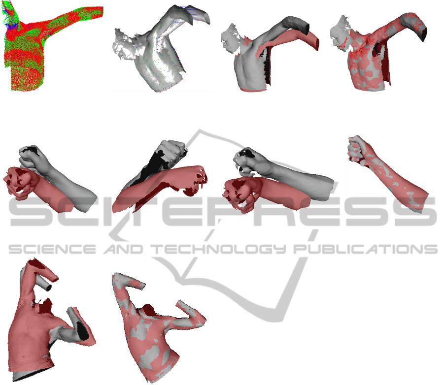
(a) CPD result (b) Correspondences (c) Before alignment (d) Result of our algorithm

Figure 6: When the CPD provides erroneous correspondences, our method can detect these outliers before it carries out the

optimization.

(a) Before alighment (view 1) (b) Before alighment (view 2) (c) Lower arm before and after deformation (d) Result of our algorithm

Figure 8: Our algorithm applied for a complex data.

(a) Before alignment (b) Result of our algorithm

Figure 7: Our algorithm simultaneously solves local de-

formation, global movement and missing data between two

surfaces.

on the target surface and the deformation provided by

the CPD result is not completely correct.

In Figure. 6, we evaluate our method on a

larger data set (N

, N

, m

) =

(71382,80762, 8540,8000, 553), an upper part of the

human body in which the deformation between two

surfaces is prominant in the area around the left shoul-

der. Moreover, near the neck, data on the source sur-

face does not exist on the target surfce. The alignment

of the CPD (Figure. 6(a)) pulls the deformed data (red

data) and align it poorly with the target data (green

data) because it matches the points around the neck

on the source data with the points around the head

on the target data. Consequently, it provides wrong

correspondences in this area. However Figure. 6(b)

shows that our method correctly detects these outliers

and removes them from the ﬁnal set of reliable corre-

spondences. Then, the proposed optimization strategy

achieves a better result for the ﬁnal alignment (Fig-

ure. 6(d)) compared to CPD.

In the next experiment, we apply our algorithm

on two surfaces with (N

, N

, m

) =

(153425,149845, 9990,9335, 731). The deformation

occurs on the entire surfaces and there is a lot of miss-

ing data between the two surfaces (Figure. 7(a)). The

algorithm deforms the source surface for ﬁnal align-

ment (Figure. 7(b)) and solves the local deformation

and global movement efﬁciently. For the missing data

on the target surface (near the left elbow), the de-

formed surface correctly aligns with the target sur-

face although there is a slight misalignment at the

top of the left elbow. This phenomenon occurs when

there are some nodes which cannot ﬁnd a correspond-

ing point in this patch, and the optimization is thus

based on the rigid energy term and the regularization

energy term for the deformation of this patch. Under

this condition, the deformation graph cannot change

rapidly enough to adapt to the abrupt change of sur-

face curvature at the elbow.

In order to demonstrate the efﬁciency of the pro-

posed method, a last experiment is carried out for

two surfaces where (N

, N

, m

)

= (48626, 45397,7930, 7981,833). The data of the

source surface (red color) and the target surface (grey

color) of the lower arm is acquired by a Creaform 3D

scanner in our lab (Figure. 8(a), 8(b)). This data is

challenging because of missing data on both two sur-

GRAPP2014-InternationalConferenceonComputerGraphicsTheoryandApplications

faces, a largely global transformation between them,

local deformation on the entire surface as well as sen-

sor noise (around the hand area). Figure. 8(c) shows

the source surface before and after deformation and il-

lustrates that our method overcomes all the challenges

of this data to deform correctly the source surface to-

ward the target surface. Final alignment between the

deformed surface and the target surface is shown in

Figure. 8(d).

5 CONCLUSIONS

We have presented an efﬁcient non-rigid registra-

tion algorithm to align two partially overlapping sur-

faces. Contrarily to other algorithms which nor-

mally require prior knowledge to obtain ﬁnal align-

ment, our method is implemented automatically with-

out any user-intervention for constraining the defor-

mation and without making other assumptions. To

achieve this, the algorithm is divided into two phases.

While the ﬁrst phase provides initial correspondences

to constrain the optimization, the strategy of the sec-

ond phase is performed in two steps in which the ﬁrst

step aims to move the source surface close to the tar-

get surface and the second step forces the two surfaces

to coincide accurately. The experimental results prove

that our algorithm can be applied to data sets where

the deformation between the two surfaces is severe

and prior knowledge is not available.

We are also aware of some limitations of our al-

gorithm. Currently, all initial correspondences are

treated equally in phase 1 without considering how

accurate they are. We need to consider the contri-

bution of each correspondence by using contribution

weights before using it in phase 2. This change may

increase convergence speed of the optimization pro-

cess in phase 2. Another limitation is related to the

deformation model. Because this model determines

the inﬂuence area of afﬁne transformations based on

Euclidean distance, this property can create strange

deformations when two nodes are close with respect

to Euclidean distance but far away with respect to

geodesic distance (two nodes of two close ﬁngers, for

example). This limitation should be considered in fu-

ture work. Once these limitations are resolved, we

plan to develop the algorithm so it can be applied for

global registration including several surfaces in order

to reconstruct a completely deformable object.

ACKNOWLEDGEMENTS

We are grateful to Myronenko et al for providing

the CPD implementation and the GRAIL laboratory-

University of Washington for providing the 3D

data. This research was supported by the NSERC-

Creaform Industrial Research Chair on 3D Scanning.

REFERENCES

Allen, B., Curless, B., and Popovi

c, Z. (2002). Articulated

body deformation from range scan data. ACM Trans.

Graph., 21(3):612–619.

Allen, B., Curless, B., and Popovi

c, Z. (2003). The space

of human body shapes: reconstruction and param-

eterization from range scans. ACM Trans. Graph.,

22(3):587–594.

Amberg, B., Romdhani, S., and Vetter, T. (2007). Optimal

step nonrigid icp algorithms for surface registration.

In Computer Vision and Pattern Recognition, 2007.

CVPR ’07. IEEE Conference on, pages 1–8.

Anguelov, D., Srinivasan, P., Pang, H.-C., Koller, D., Thrun,

S., and Davis, J. (2004). The correlated correspon-

dence algorithm for unsupervised registration of non-

rigid surfaces. In NIPS’04, pages –1–1.

Besl, P. and McKay, N. D. (1992). A method for regis-

tration of 3-d shapes. Pattern Analysis and Machine

Intelligence, IEEE Transactions on, 14(2):239–256.

Brown, B. J. and Rusinkiewicz, S. (2007). Global non-rigid

alignment of 3-d scans. ACM Trans. Graph., 26(3).

Chang, W. and Zwicker, M. (2008). Automatic registration

for articulated shapes. In Proceedings of the Sympo-

sium on Geometry Processing, SGP ’08, pages 1459–

1468, Aire-la-Ville, Switzerland, Switzerland. Euro-

graphics Association.

Chen, Y. and Medioni, G. (1991). Object modeling by reg-

istration of multiple range images. In Robotics and

Automation, 1991. Proceedings., 1991 IEEE Interna-

tional Conference on, pages 2724–2729 vol.3.

Chui, H. and Rangarajan, A. (2003). A new point match-

ing algorithm for non-rigid registration. Comput. Vis.

Image Underst., 89(2-3):114–141.

DeVore, J. (2008). Probability and Statistics for Engineer-

ing and the Sciences: Enhanced [With Glossary of

Symbols Booklet]. Available 2010 Titles Enhanced

Web Assign Series. Brooks/Cole, Cengage Learning.

Frome, A., Huber, D., Kolluri, R., Blow, T., and Malik, J.

(2004). Recognizing objects in range data using re-

gional point descriptors. In EUROPEAN CONFER-

ENCE ON COMPUTER VISION, pages 224–237.

Huang, Q.-X., Adams, B., Wicke, M., and Guibas, L. J.

(2008). Non-rigid registration under isometric defor-

mations. In Proceedings of the Symposium on Geom-

etry Processing, SGP ’08, pages 1449–1457, Aire-la-

Ville, Switzerland, Switzerland. Eurographics Associ-

ation.

Jian, B. and Vemuri, B. C. (2011). Robust point set regis-

tration using gaussian mixture models. IEEE Trans.

Pattern Anal. Mach. Intell., 33(8):1633–1645.

Non-rigidRegistrationforDeformableObjects

Johnson, A. E. (1997). Spin-images: A representation for

3-d surface matching. Technical report.

Li, H., Sumner, R. W., and Pauly, M. (2008). Global cor-

respondence optimization for non-rigid registration of

depth scans. In Proceedings of the Symposium on Ge-

ometry Processing, SGP ’08, pages 1421–1430, Aire-

la-Ville, Switzerland, Switzerland. Eurographics As-

sociation.

Madsen, K., Nielsen, H. B., and Tingleff, O. (2004). Meth-

ods for non-linear least squares problems (2nd ed.).

Mian, A., Bennamoun, M., and Owens, R. (2004). From

unordered range images to 3d models: a fully auto-

matic multiview correspondence algorithm. In Theory

and Practice of Computer Graphics, 2004. Proceed-

ings, pages 162–166.

Mitra, N. J., Fl

ory, S., Ovsjanikov, M., Gelfand, N., Guibas,

L., and Pottmann, H. (2007). Dynamic geometry reg-

istration. In Proceedings of the ﬁfth Eurographics

symposium on Geometry processing, SGP ’07, pages

173–182, Aire-la-Ville, Switzerland, Switzerland. Eu-

rographics Association.

Myronenko, A. and Song, X. (2010). Point set registration:

Coherent point drift. Pattern Analysis and Machine

Intelligence, IEEE Transactions on, 32(12):2262–

2275.

Pauly, M., Mitra, N. J., Giesen, J., Gross, M., and Guibas,

L. J. (2005). Example-based 3d scan completion.

In Proceedings of the third Eurographics sympo-

sium on Geometry processing, SGP ’05, Aire-la-Ville,

Switzerland, Switzerland. Eurographics Association.

Rusinkiewicz, S. and Levoy, M. (2001). Efﬁcient variants

of the icp algorithm. In 3-D Digital Imaging and Mod-

eling, 2001. Proceedings. Third International Confer-

ence on, pages 145–152.

Submuth, J., Winter, M., and Greiner, G. (2008). Recon-

structing animated meshes from time-varying point

clouds. In Proceedings of the Symposium on Geom-

etry Processing, SGP ’08, pages 1469–1476, Aire-la-

Ville, Switzerland, Switzerland. Eurographics Associ-

ation.

Sumner, R. W., Schmid, J., and Pauly, M. (2007). Embed-

ded deformation for shape manipulation. ACM Trans.

Graph., 26(3).

Wand, M., Adams, B., Ovsjanikov, M., Berner, A.,

Bokeloh, M., Jenke, P., Guibas, L., Seidel, H.-P., and

Schilling, A. (2009). Efﬁcient reconstruction of non-

rigid shape and motion from real-time 3d scanner data.

ACM Trans. Graph., 28(2):15:1–15:15.

GRAPP2014-InternationalConferenceonComputerGraphicsTheoryandApplications