Handling Time and Reactivity for Synchronization and Clock Drift

Calculation in Wireless Sensor/Actuator Networks

Marcel Baunach

Graz University of Technology, Institute for Technical Informatics, Graz, Austria

Keywords:

Event Timestamping, Reaction Scheduling, Time Synchronization, Clock Drift Calculation, Information

Tagging.

Abstract:

The precise temporal attribution of environmental events and measurements as well as the precise schedul-

ing and execution of corresponding reactions is of utmost importance for networked sensor/actuator systems.

Apart, achieving a well synchronized cooperation and interaction of these wirelessly communicating dis-

tributed systems is yet another challenge. This paper summarizes various related problems which mainly

result from the discretization of time in digital systems. As an improvement, we’ll present a novel technique

for the automatic creation of highly precise event timestamps, as well as for the scheduling of related (re-

)actions and processes. Integrated into an operating system kernel at the lowest possible software level, we

achieve a symmetric error interval around an average temporal error close to 0 for both the timestamps and the

scheduled reaction times. Based on this symmetry, we’ll also introduce a dynamic self-calibration technique

to achieve the temporally exact execution of the corresponding actions. An application example will show

that our approach allows to determine the clock drift between two (or more) independently running embedded

systems without exchanging any explicit information, except for the mutual triggering of periodic interrupts.

1 INTRODUCTION

Wireless sensor/actuator networks (WSAN) are com-

monly deployed to observe and interact with their en-

vironment. In this respect, temporal and spatial in-

formation are the two most fundamental measures for

the “attribution” or “tagging” of states and events (i.e.

state transitions) within any observed environment. In

this context, the states describe a set of physical and

logical conditions at a given position and at a certain

time, and they are speciﬁed by one or more continu-

ous or discrete state values.

Recorded over a certain period of time, variations

in the state values allow the detection and analysis

of events and event patterns within the environment

(Wittenburg et al., 2010) (R

omer, 2008). These vari-

ations do not only indicate the events’ spatial extend,

propagation speed, and inﬂuence on the environment,

but most commonly they also allow the prediction of

future states for both the observing system and its sur-

rounding. In this regard, the interaction with the envi-

ronment, which we already proclaimed to be the most

central objective in sensor/actuator systems, typically

requires the precise knowledge of time and space to

be associated with a node’s self-captured and exter-

nally obtained values in order to properly correlate

the contained information, and to trigger adequate re-

actions. In fact, measured or otherwise obtained en-

vironmental information is often useless unless it is

associated with temporal and spatial information.

This paper starts with a discussion of various

problems regarding time in digital systems. Next, we

present a novel approach for taking timestamps, for

measuring and specifying temporal delays, and for

scheduling and ensuring reaction times with a sym-

metric temporal error around 0. Finally, a real-world

test bed shows how periodically communicating em-

bedded systems can determine their relative clock

drifts without any additional information exchange.

2 TIME IN DIGITAL SYSTEMS

In contrast to speciﬁc position vectors and state values

of e.g. sensor nodes (which can change sporadically,

arbitrarily and independently from each other), time

is a common property. It is system independent, and

advances continuously with a globally constant rate

of change. If the sensor nodes manage to establish a

network-wide and consistent notion of time, this in-

Baunach M..

Handling Time and Reactivity for Synchronization and Clock Drift Calculation in Wireless Sensor/Actuator Networks.

DOI: 10.5220/0004680400630072

In Proceedings of the 3rd International Conference on Sensor Networks (SENSORNETS-2014), pages 63-72

ISBN: 978-989-758-001-7

 2014 SCITEPRESS (Science and Technology Publications, Lda.)

formation provides a natural base for their joint inter-

action and with the environment. Since processors in

synchronous digital systems like sensor nodes are al-

ways driven by a clock generator C with frequency f

and period λ

, time and time intervals can easily

and individually be measured – at least in theory: If it

is possible to count the number of elapsed clock peri-

ods since a well deﬁned point in time, e.g. the system

start, each captured event e, e.g. indicated by an inter-

rupt, can be attributed with its current counter value

. Consequently, the event’s absolute local system

time

can easily be recovered by

:= c

·λ

, (1)

and the time difference (i.e. the delay)

∆

between

two events e

, e

computes as

∆

−

= (c

− c

)·λ

. (2)

Obviously, both the time

and the delay

∆

al-

ready involve a concept-inherent imprecision caused

by the discretized counter values c

∈ . In addition,

we silently assumed for Eq. (1) and Eq. (2) that λ

perfectly known and constant. Neither is true under

real-world conditions, and leads to well-known prob-

lems, we’ll address and counteract in this paper.

Furthermore, as often requested for interactive

systems, a reaction r can be scheduled for a captured

event e. Its intended execution time t

∈ is com-

monly related to any event timestamp t

∈ by the

speciﬁcation of a corresponding delay ∆

e,r

∈ :

= t

+ ∆

e,r

(3)

However, in the best case, i.e. if the (operating

system) scheduler permits the timely switch to the re-

sponding task’s context, the reaction will be triggered

upon reaching the corresponding counter value c

∈

and the corresponding system time

. In any case, the

ﬁnally observable reaction delay depends on the res-

olution λ

of the system timer:

= c



∆

e,r





∆

e,r



·λ

(4)

Although the inherent rounding imprecision is

quite intuitive and introduces various hidden imple-

mentation problems in real systems, it is commonly

simply ignored. Moreover, for concurrent task sys-

tems with dynamic execution ﬂows, there is an addi-

tional error in

which is neither constant nor pre-

dictable. Since most embedded operating systems

silently accept even this problem, application devel-

opers are urged to compensate the imprecision with

little control at the task level. SensorOS (Kuorilehto

et al., 2007) at least tries to execute reactions in time

by scheduling the responsible task earlier. Yet, the

applied “delta time” is constant and won’t adapt to

changing system loads as well.

In the following we’ll indicate and discuss the

causes and effects of the mentioned problems in de-

tail, and present an approach at the kernel level to re-

liably compensate the related imprecision in the aver-

age case.

Problem P1: Discretization of time. The differ-

ence between the true global time t

and the individual

system time

t has already become visible in Eq. (1)

and Eq. (4). While the ﬁrst advances continuously,

the use of a digital counter leads to a discretization of

the latter, and imposes a resolution which directly de-

pends on the counter’s clock frequency f

. This may

lead to serious systematic errors for the time measure-

ment and the subsequent scheduling of reactions:

The simple capturing of a timestamp t for an event

– the so called timestamping – is immediately affected

by some inevitable rounding, and suffers from a mea-

surement error E

∈ I

with |I

| = λ

. For the na

ıve

and adverse reading of the timer counter, rounding

down results in I

:= [0, λ

), and induces a symmetry

around the average measurement error E

t,av

Depending on the use of such timestamps, the emerg-

ing errors might accumulate during the system run-

time. Similarly, the explicit speciﬁcation of delays

∆

in software is also subject to rounding errors E

∆

However, we can round half up (e.g. according to

DIN 1333) manually when selecting a delay, and thus

the corresponding error is E

∆

∈ I

:= [−

, +

Though not avoidable entirely, I

is at least symmetric

around 0, and the average error is 0.

Based on these two fundamental error intervals

and I

, other intervals can be derived, and con-

sequently exhibit an imprecision, too: For the mea-

surement of delays ∆

, we see the implicit compen-

sation of the asymmetry in I

: E

∆

∈ I

:= I

− I

(−λ

, +λ

). In contrast, the scheduling of reaction

times t on external events inherits the asymmetry in I

∈ I

:= I

+ I

= [−

, +

). System reactions

will consequently suffer from an average systematic

lateness of

Table 1 summarizes the error types and their cor-

responding intervals which must be expected for the

ıve capturing of timestamps by simply reading the

timer register after the corresponding event occur-

rence (e.g. within an IRQ handler). The resulting ef-

fects, and our proposed solution to compensate this

asymmetry, will be discussed later.

Problem P2: Capturing of timestamps. The cre-

ation of reactive systems demands for the precise

assignment of timestamps for internal and external

SENSORNETS2014-InternationalConferenceonSensorNetworks

Table 1: Error intervals for different discretization techniques (system time resolution: λ

ıve discretization Our discretization approach

problem / error type derived from error interval symmetry error interval symmetry

P1: capturing of fundamental I

= [0, λ

) E

E I

= [−

, +

) 0

timestamps

P2: measurement of I

− I

= (−λ

, +λ

) 0 I

= (−λ

, +λ

) 0

delays

P3: speciﬁcation of fundamental I

= [−

, +

) 0 I

= [−

, +

) 0

delays

P4: scheduling of I

+ I

= [−

, +

) E

E I

= [−λ

, +λ

) 0

reaction times

events. Reaching a voltage threshold at an analog-

digital-converter (ADC) or detecting a signal edge at

an I/O pin are just two simple examples. However,

most observable changes within the environment have

one thing in common: They are indicated to the CPU

at runtime by so called interrupt requests (IRQs), and

should be handled as soon and as fast as possible by

the corresponding interrupt service routines (ISRs).

Since ISRs are commonly higher privileged than reg-

ular application code, they will preempt the latter for

their own execution. Thus, they seem to be perfectly

suitable for capturing the timestamp for any emerging

event. However, even the ﬁrst instruction within each

ISR is not executed before some additional delay,

which is also known as interrupt latency ∆

IRQ

: If the

timer value c

for the timestamp itself is copied af-

ter another implementation-speciﬁc delay ∆

ISR

within

the ISR, then we can compute the discrete timestamp

for the captured event e as follows:

= c

·λ

− (∆

IRQ

+ ∆

ISR

) =

− ∆

(5)

Hence, a prerequisite for reliable time tracking via

Eq. (5) is, that the correction value ∆

is constant

and free from rounding errors with respect to the dis-

crete system time period. As we will see, both can be

achieved through careful code preparation.

Problem P3: Simultaneity and scheduling reliabil-

ity. Although the perfectly simultaneous transition

of two states can never occur in real systems

, the sur-

jective discretization of time can easily lead to the as-

signment of exactly the same system time for multiple

events or scheduled actions. Since resource conﬂicts

often prevent the truly parallel processing of events

as well as the simultaneous execution of (re)actions,

they usually lead to an implicit serialization. The or-

der depends on the task scheduler and the internal task

priorities. Since there is most commonly just a single

The resolution of the time measurement must simply

be chosen ﬁne enough!

IRQ controller, this is already true for the generation

of timestamps. In fact, the maximum degree of par-

allelism is always limited by the number of available

functional units

. A reliable scheduling (e.g. for com-

plying to hard real-time demands) must be achieved

through either static techniques at development time

or dynamic methods at runtime. A corresponding

technique for dynamic resource management under

real-time conditions is presented in (Baunach, 2012).

Problem P4: Imprecision in the timer frequency.

Time measurement in digital systems is usually ac-

complished by using a pulse generator with a spec-

iﬁed frequency f

. Internally, this component uses

an oscillator (most commonly a quartz crystal) to

generate a periodic clock signal. The characteristics

and stability of such oscillators depend signiﬁcantly

on their manufacturing parameters, age, and various

environmental conditions like e.g. voltage variations

(Hewlett Packard, 1997): A varying frequency drift

∆ f must always be expected. Its relative error

∆ f

is commonly expressed in units of parts per million

(ppm). For simple low-cost quartzes, and within the

typical temperature ranges of WSAN applications,

the temperature sensitivity of a typical HC49 quartz

can already result in deviations of ± 20 ppm.

Variations in the clock precision are especially

critical in distributed applications. Since time mea-

surement is initially individual for each involved sys-

tem and therefore can drift apart, this may quickly

generate inconsistent data, and must be compensated

by adequate and repeated synchronization measures.

Problem P5: Global time base and synchroniza-

tion with other systems. When does time measure-

ment actually start, i.e. when is or was time t

= 0? If

we consider a completely independent system which

uses the notion of time only for its internal operation,

Functional units refer to e.g. processors and their cores,

or to autonomously operating peripheral components.

HandlingTimeandReactivityforSynchronizationandClockDriftCalculationinWirelessSensor/ActuatorNetworks

e.g. to capture events and to schedule actions by a par-

tial order

, the use of a pure local time with arbitrary

begin is absolutely sufﬁcient – e.g. time t

= 0 may

simply indicate the system start. However, as soon

as time is of global relevance, e.g. if actions have to

take place synchronized on different systems, a com-

mon time base is often indispensable. This immedi-

ately raises the question about which time or which

system is used as reference. In any case, its provider

should be highly available and exhibit a high clock

stability and precision. Several methods exist for the

actual synchronization: Some are based on (regular)

time checks or on the measurement of the pairwise

drift between the involved systems. Others rely on

dedicated reference systems and allow the synchro-

nization based on centrally triggered events like e.g.

radio broadcasts (cf. GPS and the DCF77 protocol).

Finally, distributed methods are available for multi-

hop systems to successively achieve a common time

base, e.g. via Desynchronization (M

uhlberger, 2013).

3 AN ADVANCED TIME

DISCRETIZATION APPROACH

Considering the aforementioned problems, which

originated from the integration of time-awareness into

digital systems, P1-P3 directly affect the environmen-

tal interaction and can be addressed by each system

individually. In contrast, P4 and P5 require some

information exchange with other systems. These

“peers”, however, are not necessarily available dur-

ing the entire system runtime. For this reason, P1-P3

are treated locally at the embedded systems level (e.g.

in the operating system kernel), while P4 and P5 must

be addressed more globally (e.g. in the network layer

or at application level).

At the embedded systems level, our approach re-

lies on a hardware timer component to provide a lo-

cal system timeline with a ﬁxed temporal resolution.

The timeline management is integrated directly into

the OS kernel and accessible for all software layers

through the OS API. This uniﬁes the usage by appli-

cation tasks and avoids execution time imponderabil-

ities through unpredictable code interleaving at run-

time. Based on our approach, the kernel automat-

ically captures a timestamp

for each interrupt e,

and compensates the error’s asymmetry about

which would result from using the na

ıve approach

with I

= [0, λ

) as explained in Section 2. Therefore,

the kernel as a hardware abstraction layer provides

“Partial”, since the discretization of time may lead to

simultaneity (→ P3).

standardized and architecture dependent interrupt ser-

vice routines for introducing a constant and carefully

dimensioned delay ∆

= ∆

IRQ

+∆

ISR

before actually

capturing the timer’s counter value after the IRQ oc-

currence. According to Eq. (5) we then have to reduce

the captured counter value by an adequate correction

value ∆

corr

: Selected properly, this correction ﬁnally

results in the symmetry about 0 for I

:= [−

λ,

λ).

While the timestamp measurement error E

will still

be equally distributed over I

, this interval is shifted,

and the average timestamp error is reduced from ini-

tially

λ down to 0. At the same time, the propaga-

tion and ampliﬁcation of systematic errors for time-

dependent reactions will also be kept low and sym-

metric about 0, i.e. I

= I

+ I

= [−λ

, +λ

). Table

1 compares the error intervals of our compensation

approach with the na

ıve technique.

How can this symmetry be guaranteed? In or-

der to deal with the related problems P1 and P2, we

propose a concept based on two synchronized clocks

with interdependent frequency. Thereby, we assume

the CPU frequency to be higher than the timer fre-

quency, while conversely, the system time is derived

from the quartz-stabilized CPU clock by an even inte-

ger divider. Commonly, both requests do not impose

an unreasonable restriction on the hardware/software

design: In fact, they are already satisﬁed in many

systems, since usually only a single central oscilla-

tor is used as base for all other system clocks. While

the CPU is commonly directly driven by this main

clock, other components apply power-of-two dividers

to derive their individual frequencies. Finally, and

for computationally constrained embedded systems in

particular, driving a local time with the maximum res-

olution would cause unnecessary CPU load

Besides the following formal description of our

approach, we also refer to the example in Figure 1

for a comprehensive understanding. Initially, we de-

note the CPU clock frequency as f and its period as

λ. The system time frequency is denoted as f

and its

period as λ

. In addition, we demand for

and λ

:= α ·λ with α ∈

≥2

, α even.

(6)

If an interrupt e occurs at time t

, the corre-

sponding timer counter c

will not be copied before

some system inherent delay ∆

has passed. For our

approach, we request this delay to take exactly ∆

CPU cycles as follows:

The system time must be accumulated in software at

every timer overﬂow. Especially for timers with small word

widths, this can quickly lead to a huge performance penalty.

For instance, a 16 Bit counter counting at f

= 1 MHz will

already overﬂow after every 65.536 ms.

SENSORNETS2014-InternationalConferenceonSensorNetworks

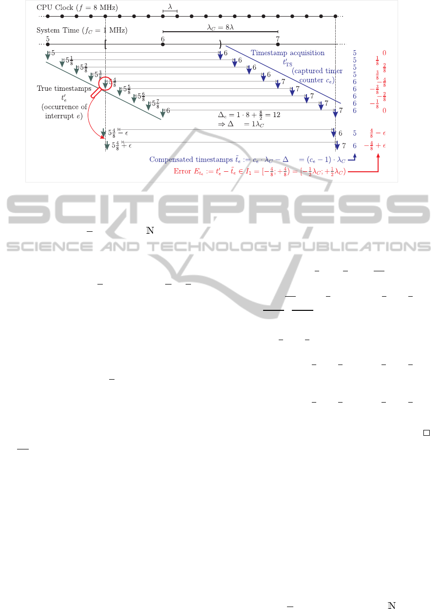
corr

Figure 1: IRQ timestamp acquisition with our approach for various potential event occurrence times t

∆

:= n·α +

with n ∈

(7)

Thus, the delayed acquisition of the timestamp takes

place at time

= t

+ ∆

= t

+ ∆

= t



n·α +



(8)

To compensate for this delay, and to force the

timestamp error interval I

to become symmetric

around the true event occurrence time while also ex-

hibiting an average error close to 0, we can select the

correction value as an integer multiple of λ

∆

corr

:= (n·α) ·

= n·λ

(9)

Thus, we simply have to subtract n from the

copied timer value c

to compute the timestamp

for

the interrupt e:





·λ

−∆

corr

= c

·λ

−n·λ

= (c

− n) ·λ

(10)

Since c

(timer driven) and n (constant) are inte-

gers of architecture word width, their subtraction is

easily accomplished. Besides, the result’s resolution

implicitly equals the resolution of the system time.

However, we still have to prove the symmetry about 0

for the error intervals in Table 1:

Lemma 1. For our discretization approach the error

intervals I

, I

, and I

for taking timestamps, for

measuring and specifying delays, as well as for com-

puting reaction times are symmetric about 0.

Proof. While I

is not affected by our novel approach,

the demanded symmetry of I

, I

, and I

can easily be

proofed by some interval arithmetic. With Eq. (8),

(10) the expected error E

of the timestamp

com-

putes as

= t

−



−



n·α +

·α





−





·λ

− n ·λ



= t

−





·λ

| {z }

∈[0,λ

)

−

·λ

∈



−

, +



⇒ I



−

, +



⇒ I

= I

− I



−

, +



−



−

, +



= (−λ

, +λ

)

⇒ I

= I

+ I



−

, +





−

, +



= [−λ

, +λ

)

3.1 An Implementation Example

As an example, we’ll take a look at the integration

of our novel approach into the reference implemen-

tation of SmartOS (Baunach et al., 2007) for the

MSP430F1611 (Texas Instruments Inc., 2006) MCU

and the SNoW

sensor nodes (→ Figure 1) . While

the main clock drives the CPU at f = 8 MHz, the di-

vider α = 8 derives the frequency f

= 1 MHz for the

system time with a resolution of 1 µs. According to

Eq. (7), an adequate delay ∆

between each interrupt

occurrence and the acquisition of its timestamp can

be adjusted through n:

∆

:= n·α +

= n·8 + 4 with n ∈

(11)

HandlingTimeandReactivityforSynchronizationandClockDriftCalculationinWirelessSensor/ActuatorNetworks

1 _ _ i r q_e:

2 ; hardw a r e IRQ l a t e nc y ; +6 CPU cycle s f r o m t

∆

IRQ

= 6λ

3 nop ; +1 CPU cycle \

4 nop ; +1 CPU cycle > ∆

ISR

= 6λ

5 mov & T I M ER_ C O U NTE R , & TS ; +4 CPU cycl e s f o r l a t c h in /

6 ; T otal d e l a y of c a ptu r e d t im e s ta m p : ∆

= ∆

IRQ

+ ∆

ISR

= 12λ = 1.5µs

8 mov #e , & _ _i r q_ n um b e r ; save IRQ num b e r for su b s eq u en t pr o ce s s in g in the as s oc i a te d even t h an d l e r

9 jmp __ k e r n e l _ en t ry ; j u m p to ke r n e l code

Listing 1: Timestamping within a specially prepared kernel ISR for IRQ number e.

Listing 1 shows the standardized kernel ISR for any

interrupt with number e: Since the CPU inherently de-

lays the acceptance of an interrupt by ∆

IRQ

= 6 CPU

cycles, we already have to select n ≥ 1. In fact, we

did select n = 1 and thus have to wait for an additional

number of ∆

ISR

:= ∆

− ∆

IRQ

= 6 CPU cycles within

the ISR (1 · 8 + 4 = 6 + 6). According to the speciﬁ-

cation of the mov instruction, which is used for saving

the timer value TS in Line 5, it takes 4 CPU cycles

until the value is read from the special function reg-

ister TIMER COUNTER. The remaining two cycles are

ﬁlled up by nop instructions. After the acquisition of

the counter value, the speciﬁc IRQ number is saved

and the kernel mode is entered for the actual event

handling.

To save CPU time the ISR will only save the cur-

rent 16 Bit timer value which indicates the delay since

the last timeline update. The computation of the ﬁnal

absolute timestamp

is initially avoided, and delayed

until the application’s event handler requests this in-

formation from the OS. Then, according to Eq. (9), n

is simply subtracted from the event’s absolute counter

value c

, which in turn is the sum of the timeline and

the just captured timer value TS. With Eq. (10) the

result can directly be interpreted as absolute system

time given in the timeline resolution of 1 µs:

= (c

− n)·λ

= (timeline + TS − n)·λ

(12)

Note that the applied computation is correct, as long

as the IRQ handlers are always executed in kernel

mode where further interrupts are disabled and nei-

ther the timeline nor TS will change concurrently.

4 EVALUATION AND

APPLICATION EXAMPLE

The test bed for demonstrating the beneﬁt of our

timestamping approach consists of pairs of nodes A, B

playing some sort of Ping Pong game as depicted in

Figure 2: By a wired or wireless remote connection,

one node, WLOG B, triggers an IRQ signal e

which

is received and timestamped (

) by the other node

A through the just presented timestamping approach.

After some ﬁxed delay ∆

delay

the signal will be re-

turned by node A, and in turn the other node B catches,

timestamps, and returns the signal after the same de-

lay ∆

delay

. Having received the last trigger e

with lo-

cal timestamp

in a perfect system, the observed de-

lay

∆

total,n

between each node’s captured ﬁrst and last

signal timestamp should obviously equal the mathe-

matically expected delay ∆

total,n

∆

total,n

−

= 2n·∆

delay

=: ∆

total,n

(13)

However, this equality will commonly not be ob-

servable in real systems. In fact each involved device

will suffer from its own and the other device’s impre-

cision:

First, the nodes apply independent clocks, drift

apart, and, though globally ﬁxed, they will ﬁnally not

defer their responses by exactly the same delay ∆

delay

Though our nodes’ CPUs are driven by quartzes from

the same lot, the clock drifts vary depending on the

selected node pair and the environmental inﬂuences

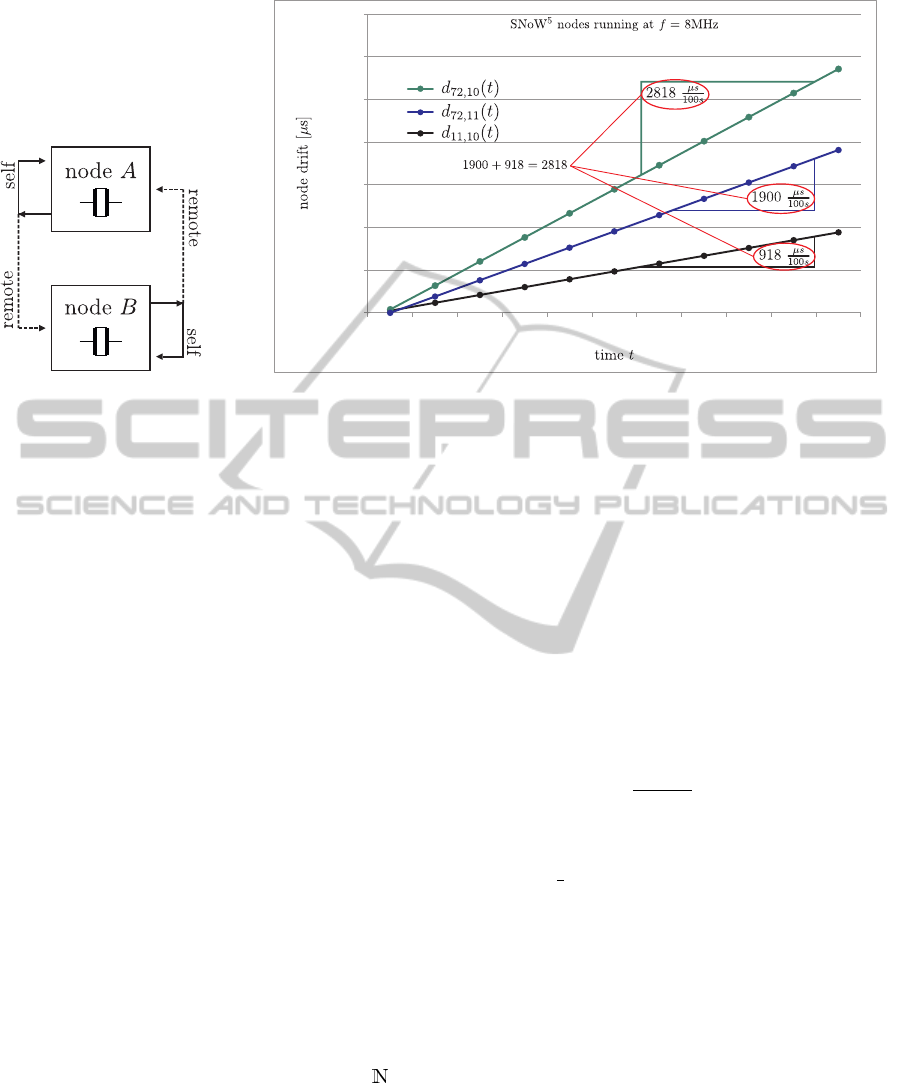
described before. In fact, Figure 3 shows signiﬁcantly

different drifts d

A,B

(t) for three node pairs measured

over some time t.

Second, the responses must be scheduled and ini-

tiated by the responsible task on each node. There-

fore, these tasks compute their next intended local re-

sponse time t

∗

from each previously captured signal

timestamp, and then sleep to release the CPU for other

tasks. However, waking up sufﬁciently early to emit

the signal in time is not that easy since some load-

dependent and variable system overhead must always

be taken into account.

Third, the base for each delay computation is

never perfect since each captured timestamp

ex-

hibits an inherent error E

∈ I

. While this cannot be

The nodes with IDs 10, 11, and 72 were arbitrarily se-

lected from our pool. The drift was measured via an oscillo-

scope tracking the delay between two periodically triggered

I/O pins at both nodes of each pair. As a plausibility test,

the measured drift of each pair corresponds perfectly to the

other pairs’ drifts: 918

µs

100s

+ 1900

µs

100s

= 2818

µs

100s

SENSORNETS2014-InternationalConferenceonSensorNetworks

trigger

Figure 2: The Ping Pong test

bed setup (remote connections

can be wired or wireless).

256

1175

2094

3013

3932

4851

5767

6682

7599

8515

9431

5000

10000

15000

20000

25000

30000

35000

0 100 200 300 400 500 600 700 800 900 1000

400

3181

6021

8839

11660

14480

17300

20120

22940

25760

28580

160

2060

3960

5862

7763

9662

11563

13463

15364

17264

19165

Figure 3: Clock drift for three node pairs.

avoided entirely as discussed before, the error should

at least be about 0 µs in the average case according to

Lemma 1.

4.1 Signal TX and Self-Calibration

For the precisely timed signal emission, we pro-

pose a dynamic self-calibration scheme based on self-

observation. Therefore, the trigger signal will not

only be captured by the other node where it is tagged

with the timestamp

, but also by the emitting node it-

self. We denote the corresponding local timestamp as

. If the intended local response time for the current

iteration has been computed as t

∗

, the lateness can be

computed afterwards and used as compensation value

∆

comp

to adjust the delay for the next iteration at its

emission time t

∗

∆

comp

−t

∗

(14)

∗

+ ∆

delay

− ∆

comp

(15)

In fact, the response time precision error (E

∗

∈

) depends not only on the two timestamps and their

particular precision error (E

, E

∈ I

), but also on the

error in the measured delay (E

∆

comp

∈ I

) and the hard

coded delay for the reply (E

∆

delay

∈ I

) itself. Since we

intentionally selected ∆

delay

:= m ·λ

with m ∈ , at

least this value is free from rounding errors and I

[0;0) for this special application.

4.2 Pairwise Drift Calculation

For our tests we set up various node pairs A and B as

depicted in Figure 2, and we were interested in each

nodes’ x ∈ {A, B} local timing error e

which was au-

tonomously calculated by each node after n iterations:

Eq. (13)

∆

total,n

−∆

total,n

= (

−

)−2n · ∆

delay

(16)

Obviously, both timing errors e

, e

have different

sign unless the clocks are perfectly synchronous (then

= e

= 0 µs). Additionally, we deﬁne the symme-

try error e

symm

as seen by an external observer as the

average value over e

, e

. Since the average times-

tamp error E

t,av

∈ I

will accumulate over the two ac-

quired trigger timestamps within each iteration, we

expect

symm

+ e

= 2n·E

t,av

. (17)

If we indeed achieved the timestamp error in-

terval I

to be symmetric about 0, i.e. by selecting

∆

= n · α +

·α properly according to Eq. (7), we can

expect two observations for any pair of nodes A, B:

1. If both values e

and e

are made available to an

external observer, their measured clock drift d

A,B

as depicted in Figure 3, can be veriﬁed through

A,B

:= e

−e

= d

A,B

with d

A,B

= −d

B,A

(18)

2. According to Eq. (17), e

symm

= 2n · 0µs = 0µs, and

thus both values e

and e

will show the same ab-

solute values. In direct consequence, each node

can autonomously estimate its own drift towards

the other node autonomously:

A,B

= 2·e

(for node A) (19)

B,A

= 2·e

(for node B) (20)

HandlingTimeandReactivityforSynchronizationandClockDriftCalculationinWirelessSensor/ActuatorNetworks

-1500

-1000

-500

500

1000

1500

10 11 12 13 14 15 16 17 18

time errors [µs]

symm

1483.3

71.8

-1339.7

d’ =

2823.0

1397.3

-13.7

-1424.7

d’ =

2822.0

1407.6

-0.7

-1409.0

d’ =

2816.6

1430.0

10.5

-1409.0

d’ =

2839.0

1440.7

23.2

-1394.3

d’ =

2835.0

1454.3

34.5

-1385.3

d’ =

2839.7

1461.4

49.5

-1362.4

d’ =

2823.8

1474.3

60.0

-1354.3

d’ =

2828.5

1484.8

71.9

-1341.0

d’ =

2825.8

Expected: 0.0 Expected: 50.0

Expected: 2818

-1500

-1000

-500

500

1000

1500

10 11 12 13 14 15 16 17 18

time errors [µs]

symm

1024.7

70.0

-884.7

d’ =

1909.3

924.3

-15.2

-954.7

d’ =

1879.0

950.3

-0.4

-951.0

d’ =

1901.3

965.0

10.5

-944.0

d’ =

1909.0

997.7

24.2

-949.3

d’ =

1947.0

995.7

34.5

-926.7

d’ =

1922.3

1016.0

49.0

-918.0

d’ =

1934.0

1016.0

61.8

-892.3

d’ =

1908.3

1030.3

70.3

-889.7

d’ =

1920.0

Expected: 0.0 Expected: 50.0

Expected: 1900

-1500

-1000

-500

500

1000

1500

10 11 12 13 14 15 16 17 18

time errors [µs]

∆

[λ]

symm

539.5

71.4

-396.8

d’ =

936.3

443.0

-15.3

-473.5

d’ =

916.5

458.0

-0.5

-459.0

d’ =

917.0

468.8

9.3

-450.3

d’ =

919.0

492.8

23.6

-445.5

d’ =

938.3

497.8

35.5

-426.8

d’ =

924.5

516.5

48.3

-420.0

d’ =

936.5

526.8

60.8

-405.3

d’ =

932.0

531.3

71.6

-388.0

d’ =

919.3

Expected: 0.0 Expected: 50.0

Expected: 918

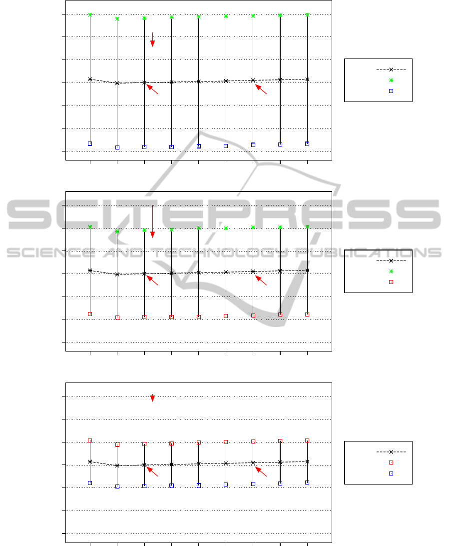
Figure 4: The node timing error for different values of ∆

after 100 s as autonomously measured by each node (see Figure 3

for the expected values).

SENSORNETS2014-InternationalConferenceonSensorNetworks

Table 2: Drift calculation for ∆

= 12.

local information

1,2

observer

A,B

node 10 node 11 node 72 d

A,B

72,11

1900.0 1902.0 1900.0 1900

72,10

2818.0 2818.0 2816.0 2818

11,10

918.0 916.0 916.0 918

regular font: measured according to Eq. (19)

bold/italic: derived according to Eq. (21)

true drift as expected from Figure 3

Table 3: Drift calculation for ∆

= 16.

local information

1,2

observer

A,B

node 10 node 11 node 72 d

A,B

72,11

1884.0 1836.0 2032.0 1900

72,10

2724.0 2870.0 2922.0 2818

11,10

840.0 1034.0 890.0 918

regular font: measured according to Eq. (19)

bold/italic: derived according to Eq. (21)

true drift as expected from Figure 3

In particular, the exchange of any additional data,

such as timestamps, between the nodes is not nec-

essary to obtain this information (since ∆

delay

constant).

The reason becomes clear when considering the

involved error intervals over n iterations in Eq. (24):

Obviously, all error intervals remain symmetric about

0 µs throughout the entire test. In particular, the aver-

age error for each variable is 0 µs, and consequently

symm

= 0 µs, too.

In contrast, if we intentionally violate Eq. (7) by

using e.g. ∆

:= n·α instead, the average times-

tamp error interval would be symmetric around E

. Consequently, e

symm

= 2n ·

, and neither the

autonomous drift computation through Eq. (19) nor

the external drift veriﬁcation through Eq. (18) would

work any more.

4.3 Real-World Test Bed Analysis

Figure 4 shows the test bed results for the three al-

ready mentioned node pairs from Figure 3, and for

various values of ∆

after n = 50 iterations with

∆

delay

= 1 s (∆

total,n

= 100 s). Note that the results

repeat in a cyclic manner with period α = 8, and thus

the values for ∆

= 10 are similar to those for ∆

= 18.

When using ∆

= 1 ·8 +

= 12, we did indeed

achieve the expected symmetry error e

symm

≈ 0 µs

for all pairs. At least we received |e

symm

| < λ

1 µs, which is the timeline resolution and thus the best

timestamp precision a node can reach. Furthermore,

for ∆

= 12, d

A,B

≈

A,B

veriﬁes the measured values

from Figure 3. Most important, as shown in Table 2,

the autonomously measured drifts between two nodes

are almost perfect. Indeed, the maximum visible de-

viation is in range ±2 µs. Another fact which we can

verify from this table is, that since WLOG node A

knows its drifts

A,B

and

A,C

towards the two other

nodes B and C respectively, it can also reliably derive

the drift

B,C

via

B,C

A,C

−

A,B

. (21)

For any other values of ∆

violating Eq. (7), the

nodes can not gain reliable information about their

relative drift autonomously. When using e.g. ∆

2·8 = 16, Figure 4 shows values close to the ex-

pected symmetry error e

symm

= 2n ·

= 50 µs (cf.

Eq. (17)). As a result, Table 3 summarizes the au-

tonomously measured and computed drifts between

the node pairs, and reveals quite large and asymmet-

ric deviations towards the true drifts.

Besides the precision of the autonomous drift esti-

mation, another interesting metric is the resulting trig-

ger frequency. The theoretical value

trig



2·∆

delay



−1

(22)

will not be visible in reality since neither node uses

a perfect clock. However, we would at least like to

achieve

trig, av.



∆

delay,A

+ ∆

delay,B



−1

, (23)

which is deﬁnitely the best compromise two nodes

A, B can ﬁnd if their true drift compared to the perfect

global clock is unknown. Again, this is only possible

if e

symm

= 0. When looking at e.g. the graph for the

nodes with IDs 11 and 72 in Figure 4, the extrapola-

tion of e

symm

leads to a symmetry error of −345.6 µs

for ∆

= 12 and 42336 µs for ∆

= 16 within one com-

plete day. Thus, the larger |e

symm

| the larger the de-

viation from the intended frequency f

trig, av.

. The ef-

fects are once more visible in Tables 2 and 3: For

∆

= 12 the values in each row are almost equal (i.e.

consistent), while they exhibit signiﬁcant variations

for ∆

= 16.

5 CONCLUSIONS AND

OUTLOOK

In this paper we proposed an approach for obtaining

precise timestamps

for external events e, and for

ensuring the precisely timed execution of reactions

r at scheduled times

. The error intervals for both

HandlingTimeandReactivityforSynchronizationandClockDriftCalculationinWirelessSensor/ActuatorNetworks

∗

Eq. (15)

+ ∆

delay

− ∆

comp

iteration I

1 : [−λ

;λ

) [−

;

) [0;0) (−

;

)

n : [−nλ

;nλ

) [−

;

) [0;0) (−(n −

)λ

;(n −

)λ

)

∆

comp

Eq. (14)

− t

∗

iteration I

1 : (−

;

) [−

;

) [−λ

;λ

)

n : (−(n +

)λ

;(n +

)λ

) [−

;

) [−nλ

;nλ

)

(24)

and

are symmetric about 0. While the ﬁrst is

achieved through the uniﬁed and carefully prepared

preprocessing of interrupts by the kernel, the latter

becomes possible through a simple self-calibration

scheme at application layer. Both techniques proved

to be a great beneﬁt for an inherent problem within

distributed but interacting (embedded) systems: As

long as time is not properly manageable locally by

the individual nodes, network-wide synchronization

and event or state tagging will hardly achieve the po-

tentially feasible precision.

Using our approach, a corresponding test bed ver-

iﬁed, that it is possible to determine the drift be-

tween two nodes without the explicit exchange of any

quantitative information (like e.g. timestamps or pre-

viously measured delays). Instead, it is sufﬁcient to

periodically pass events (i.e. interrupts) between the

nodes. Since suitable periodic behavior can also be

found in several (wireless) communication protocols

like (Støa and Balasingham, 2011), (Ito et al., 2009),

(Mutazono et al., 2009), the proposed techniques can

also be applied to support time synchronization and

self-organization among the involved systems.

In fact, we already observed good time synchro-

nization results when integrating our approach into

the Desync protocol from (M

uhlberger, 2013). An-

other objective for us is to support our timestamping

concept in hardware: Within a hardware/software co-

design project, a speciﬁcally prepared interrupt con-

troller of an experimental CPU architecture is already

able to pre-process and store timer values even for si-

multaneously occurring events.

REFERENCES

Baunach, M. (2012). Towards Collaborative Resource Shar-

ing under Real-Time Conditions in Multitasking and

Multicore Environments. In 17th IEEE International

Conference on Emerging Technology & Factory Au-

tomation (ETFA 2012). IEEE Computer Society.

Baunach, M., Kolla, R., and M

uhlberger, C. (2007). Intro-

duction to a Small Modular Adept Real-Time Operat-

ing System. In 6. GI/ITG KuVS Fachgespr

ach Draht-

lose Sensornetze. RWTH Aachen University.

Hewlett Packard (1997). Fundamentals Of Quartz Oscilla-

tors. Electronic Counters Series.

Ito, K., Suzuki, N., Makido, S., and Hayashi, H. (2009). Pe-

riodic Broadcast Type Timing Reservation MAC Pro-

tocol for Inter-Vehicle Communications. In 28th IEEE

conference on Global telecommunications (GLOBE-

COM 2009). IEEE Press.

Kuorilehto, M., Alho, T., H

annik

ainen, M., and

ainen, T. D. (2007). SensorOS: A New Oper-

ating System for Time Critical WSN Applications. In

7th International Workshop on Embedded Computer

Systems (SAMOS 2007), LNCS. Springer.

uhlberger, C. (2013). On the Pitfalls of Desynchro-

nization in Multi-hop Topologies. In 2nd Inter-

national Conference on Sensor Networks (SENSOR-

NETS 2013). SciTePress.

Mutazono, A., Sugano, M., and Murata, M. (2009). Frog

Call-Inspired Self-Organizing Anti-Phase Synchro-

nization for Wireless Sensor Networks. In 2nd Inter-

national Workshop on Nonlinear Dynamics and Syn-

chronization (INDS 2009).

omer, K. (2008). Discovery of Frequent Distributed Event

Patterns in Sensor Networks. In 5th European Con-

ference on Wireless Sensor Networks (EWSN 2008).

Støa, S. and Balasingham, I. (2011). Periodic-MAC: Im-

proving MAC Protocols for Wireless Biomedical Sen-

sor Networks through Implicit Synchronization. In

Biomedical Engineering, Trends in Electronics, Com-

munications and Software. InTech.

Texas Instruments Inc. (2006). MSP430x161x Mixed Signal

Microcontroller. Dallas (USA).

Wittenburg, G., Dziengel, N., Wartenburger, C., and

Schiller, J. (2010). A System for Distributed Event

Detection in Wireless Sensor Networks. In 9th

ACM/IEEE International Conference on Information

Processing in Sensor Networks (ISPN2010).

SENSORNETS2014-InternationalConferenceonSensorNetworks