
Map-based Lane and Obstacle-free Area Detection
T. Kowsari, S. S. Beauchemin and M. A. Bauer
Department of Computer Science, The University of Western Ontario, London, ON, N6A-5B7, Canada
Keywords:
Lane Detection, Stereo Vision, Particle Filters, Lane Maps.
Abstract:
With the emergence of intelligent Advanced Driving Assistance Systems (i-ADAS), the need for effective
detection of vehicular surroundings is considered a necessity. The effectiveness of such systems directly
depends on their performance in various environments such as rural and urban roads, and highways. Most of
the current lane detection techniques are not suitable for urban roads with complex lane shapes and frequent
occlusions. We propose a map-based lane detection approach which can robustly detect the lanes in urban and
rural environments, and highways. We also present an algorithm for detecting obstacle-free areas in detected
lanes based on the stereo depth maps of driving scenes. Experiments show that our approach reliably detects
lanes and obstacle free areas within them, even in case of partially occluded or worn-off lane markers.
1 INTRODUCTION
Today, almost every new vehicle has some form
of Advanced Driving Assistance System (ADAS).
From adaptive cruise control, collision avoidance, and
lane crossing warning systems to parking assistance,
ADAS has made driving a safer and more enjoyable
task. While a simple driving assistance system still
requires a wealth of information on the state of the
vehicle and its relationship to the immediate environ-
ment, intelligent ADAS requires even more, including
information on the state of the driver. Furthermore,
the relative position and speed of other vehicles (and
obstacles) constitute essential informational elements
in the determination of lane-based safe and driveable
areas directly located in front of the vehicle. In this
contribution, we present an innovative lane detection
system which combines GPS informationand a global
lane map with a forward facing vehicular stereo sys-
tem to achieve robust lane detection. In addition, the
stereo depth map enables the detection of lane-based,
obstacle-free areas.
Lane detection may appear trivial, at least in its
basic setting. For instance, a relatively simple Hough
transform-based algorithm can be used to detect the
host lane for a short distance ahead without any track-
ing. This method proves effective in roughly 90%
of the highway cases (Borkar et al., 2009). How-
ever, lane detection is considered a very challenging
task when lanes other than the host one, obstacles
of all kinds, and sharp turns are taken into account.
The absence of lane markers (or worn-off ones), var-
ious lane shapes and sizes, occlusion, illumination
changes, and weather conditions are among the rea-
sons why lane detection is not as simple as it seems.
A recent lane and road boundary detection survey
(Hillel et al., 2012) explored a large body of research
on lane detection, including methods using gradient-
based feature detection (Samadzadegan et al., 2006;
Nieto et al., 2008; Sawano and Okada, 2006), steer-
able filters (McCall and Trivedi, 2006), box filters
(Huang et al., 2009; Wu et al., 2008), and learning-
based lane pattern recognition (Cheng et al., 2006).
Lane models, such as straight lines (Kim, 2008;
Pomerleau, 1995; Rasmussen and Korah, 2005),
parabolic curves (Huang et al., 2009; McCall and
Trivedi, 2006), semi-parametric formulations such as
splines (Kim, 2008), or active contours (Sawano and
Okada, 2006) are found in the literature. Differ-
ent model-fitting methods have been adopted includ-
ing RANSAC (Sawano and Okada, 2006), particle
swarms (Zhou et al., 2005), energy-based optimiza-
tion (Sawano and Okada, 2006), genetic algorithms
(Samadzadegan et al., 2006), and more. Despite this
vast body of research, there are problems which yet
remain to be satisfactorily addressed:
• Lane markings cannot be detected with range
finders or other types of sensing that do not pro-
vide visible spectrum images. Even when sen-
sors are adapted to lane marking detection, exter-
nal problems arise, such as adverse weather, weak
illumination, and worn-off markings, among oth-
ers. Only a few authors in the literature have used
specialized sensors such as line sensors (Narita
et al., 2003) or GPS (Jiang et al., 2010) to as-
sist the detection process. In this contribution we
523
Kowsari T., S. Beauchemin S. and A. Bauer M..
Map-based Lane and Obstacle-free Area Detection.
DOI: 10.5220/0004675005230530
In Proceedings of the 9th International Conference on Computer Vision Theory and Applications (VISAPP-2014), pages 523-530
ISBN: 978-989-758-009-3
Copyright
c
2014 SCITEPRESS (Science and Technology Publications, Lda.)

demonstrate how GPS and vehicle speed obtained
from the internal network of the vehicle (CAN-
bus) may be used in the design of a robust lane
detection algorithm.
• Except in a few instances (Kim, 2008; Huang
et al., 2009), in almost the entire lane detection
literature, lane models are not taking splitting and
merging lanes (such as left turn lanes or open-
ing and closing lanes) into account. Models often
consist of parallel lanes without any distortion or
starts and end to them. We have used a very sim-
ple yet flexible way of representing lanes such that
all types of lanes can be represented and detected
in most situations.
• Current lane detection algorithms are usually de-
signed and tested either on highways or rural
roads where sharp changes in lane position and
orientation are not often observed. Our ap-
proach was tested successfully in dense urban
areas where sharp turns, vehicle clutters, lane
marker coverage, buildings, or other urban ar-
tifacts distract conventional lane detection algo-
rithms.
• Most times, the most important lane from the
point of view of the detection process is the host
lane. However, in some cases we are interested
in being able to describe a more complex environ-
ment such as the sum of lines adjacent to the host
one.
We first provide a map-based framework which
uses the GPS, vehicular speed, and a pre-loaded digi-
tal lane map as inputs to the lane detection algorithm.
We then present the lane feature detection mechanism
together with a particle swarm based tracking algo-
rithm which fits the map with the lanes in the images.
Subsequently, we use a simple yet effective stereo
depth-based obstacle detection by which we find the
obstacle-free lane areas in front of the vehicle.
This contribution is organized as follows: Sec-
tion 2 introduces the global lane map and lane mod-
eling, Section 3 provides lane features and the Parti-
cle Swarm Optimization (PSO) algorithm, Section 4
describes the obstacle detection mechanism and the
method to compute the obstacle-free lane areas, Sec-
tion 5 presents the experimental results, and Section 6
offers a conclusion.
2 LANE MODEL
We present a global lane model for lane detection.
While this type of model is not very common in the
literature, we believe that it provides key advantages
to the development of robust lane detection mecha-
nisms. Using a lane map containing all lane paths
and vehicle location on that map (with GPS or other
methods for localization) facilitates the lane detection
process and results in a more robust approach to the
problem. To form the required lane maps, we anno-
tated lanes in images provided by Google Earth satel-
lite imagery.
In most of the methods found in the existing lit-
erature, it is generally assumed that the lane markers
on the ground plane are approximately parallel. How-
ever, in reality, lane markers do not conform to this as-
sumption. Even on roads where there is no splitting or
merging of lanes, there are frequent lane shape distor-
tions. In addition, most methods are concerned with
the detection of the host lane only. We propose that
modeling multiple lanes can significantly contribute
to the robustness of lane detection algorithms, as any
detectable part of a lane assists in preserving stabil-
ity, especially in the absence of other cues. In light of
this, it is believed that a robust model should have the
following properties:
• The model should address the observed shapes of
lanes.
• In addition to the detection of the host lane, the
model should be able to detect visible adjacent
lanes.
• The model should include splitting and merging
lanes (for instance, left turn lane parts in the center
of the road at intersections or highway merging
lanes)
The model contains a number of splines which
model the entire map of the region of interest. Each
spline is a lane marker and consists of points whose
absolute positions on the map are their GPS latitude
and longitude. In addition, these splines are binned
into grid buckets representing non-overlapping con-
tiguous regions each 500m
2
in size. The sum of these
buckets cover the entire lane map.
Each time the vehicle records data (it does so at
30Hz), a search for spline buckets that are most prob-
ably visible occurs, given the vehicle’s position and
orientation, and the front stereo system viewingangle.
The lane marking splines from the selected buckets
are subsequently sorted in space with respect to the
perpendicular of the direction of the vehicle, which
amounts to a sorting from left to right in terms of vis-
ibility from the point of view of the stereo system.
With t sorted lane marking splines hypothetically
forming t −1 lanes and two out-of-road areas, and
the position (latitude and longitude) and orientation
(obtained with the vector formed from the last two
GPS coordinates) of the vehicle, the positions of the
VISAPP2014-InternationalConferenceonComputerVisionTheoryandApplications
524

Figure 1: Images from the map building application a)
(left): Splitting lanes b) (right): Several neighboring lanes.
splines are converted into the reference frame of the
front stereo system (with its origin at the optical cen-
ter of the left camera) in meter units. Each lane
L
i
∈{L
0
,...,L
t−1
} is composed of two lane marking
splines.
In order to specify the modalities of splitting and
merging lanes, the model requires the opening and
closing distances of the lanes from the vehicle. To ad-
dress this, at each time interval, we assign t −1 vari-
ables LaneCloses(i) for the closing distance of each
lane and another t −1 variables LaneOpens(i) with
the same size for the opening distance of each lane.
The opening distances for the lanes which are already
open are set to 0, while the closing distances for the
lanes that are not yet closed are set to ∞.
Since we require our model to detect obstacle-free
areas in the lanes, we considered another t + 1 vari-
ables LaneBlocks(i) which contain either ∞ to sig-
nify not blocked or a distance in meters indicating that
there is an obstacle in this lane at that distance.
2.1 Spline Lane Marker Model
We adopted the Catmull-Rom spline formalism for
the lane-marking splines (Catmull and Rom, 1974)
since it interpolates the control points. For each spline
segment between control points P
i
and P
i+1
, the spline
is obtained with control points P
i−1
to P
i+2
as (Watt
and Watt, 1991):
S(t) =
1 t t
2
t
3
M
P
i−1
P
i
P
i+1
P
i+2
(1)
where S(t) is either the x or y element of the coordi-
nates of the curve points, t ∈ [0, . . . ,1] and
M =
1
2
0 2 0 0
−1 0
1
2
0
2 −5 4 −1
−1 3 −3 1
2.2 Generating the Lane Map
Google Earth satellite images are used to build the
lane maps. Satellite images adequately fit our pur-
poses as lane markers are not occluded by vehicles
or other urban structures. These images can also be
addressed directly by longitude and latitude which is
desirable since we use GPS coordinates to locate the
vehicle on the map and extract hypothetically visible
lanes from the stereo images. We created an applica-
tion which uses Google static API to obtain and dis-
play bird’s eye images of the region of interest at re-
quested positions. (see Figure 1). This application
also allows a user to draw and edit splines as lane
markers. The user is also able to navigate through the
map and follow the road while drawing lanes. The re-
sulting data is saved as a set of lane-marking splines,
each of them containing a set of control points. In our
experiments, we extracted a path that was traveled by
the experimental vehicle within the city of London,
Ontario. This path consists of 94 lanes and lane seg-
ments, including right and left turn lanes.
3 MODEL FITTING USING A
PARTICLE FILTER
With the knowledge of the position and orientation of
the vehicle within the lane map, we proceed to fit our
lane model onto the detected lane features in the left
stereo image.
Since the GPS data frequency (1Hz) is signif-
icantly slower than that of the front stereo system
(30Hz), the most recent speed data of the vehicle ob-
tained from the CANBus is used to extrapolate the
most recent available GPS data to coincide with the
most recent image frame from the front stereo sys-
tem. This can be thought as a form of synchroniza-
tion of the GPS device and the front stereo system. In
addition, the GPS data has a relatively large error (we
observed a ±5m error), and can be used only as a seed
for the lane fitting process.
With the approximate position and orientation of
the vehicle, the visible parts of the lane map in the
image can be identified. The lane-marking splines
are projected onto the stereo left image and an opti-
mization algorithm attempts to find the best relative
change in the position and orientation of the vehicle
which best fits the projection with the lane features in
the image. This optimization yields two parameters
δX and δθ which correct the current vehicle position
and orientation obtained form the GPS at each frame.
In order to project the lane markers onto the image
we need to know the ground plane equation parame-
Map-basedLaneandObstacle-freeAreaDetection
525

ters in the camera coordinate system. Even though the
ground plane parameters are very stable, we noticed
that including a correction parameter δλ representing
the difference between the ground plane and the x,z
plane of the stereo camera system improves the accu-
racy of the projection process by compensatingfor the
unexpected tilt variations due to vehicle suspension.
3.1 Ground Plane Estimation
The ground parameters needed for projecting the
lanes on the image can be computed from the depth
map obtained from the stereo system. With rec-
tified stereo images, finding disparities and hence
depth map merely consists of a 1-D search with a
block matching algorithm (our implementation uses
the stereo routines from Version 2.4 of OpenCV) As-
suming that the ground plane equation is of the form
ax+ by+ cz = d (2)
where ~n = (a, b,c) is the unit normal vector to the
plane, we pose
d =
1
√
a
′2
+ b
′2
+ c
′2
(3)
a
b
c
= d
a
′
b
′
c
′
(4)
With the coordinates of 3D points in the reference sys-
tem of the left camera
(X
i
,Y
i
,Z
i
) (5)
we can write
Ax = B (6)
and solve for x in the least-squares sense as
x = (A
T
A)
−1
A
T
B (7)
where
A =
X
1
Y
1
Z
1
X
2
Y
2
Z
2
.
.
.
.
.
.
.
.
.
X
n
Y
n
Z
n
B =
1
1
.
.
.
1
x =
a
′
b
′
c
′
Often times the ground surface leads to inordinate
amounts of outliers, due in part to a lack of tex-
ture from the pavement or other driveable surfaces.
With the sensitivity of least-squares to outliers being
known, we resort to the use of RANSAC in select-
ing the inliers and obtain a robust estimation of the
ground plane coefficients, in the following way:
1. randomly select three points from the 3D points
believed to be representative of the ground plane
2. compute the coefficients of the plane defined by
the randomly selected points using (6)
3. count the points whose distance to the plane is less
than a threshold ε
4. repeat these steps n times where n is sufficiently
large
1
5. among the n fits choose the largest inlier set which
respect to ε and compute the coefficients of the
ground plane this time using least-squares as in
(7)
The plane parameters are averaged over a short period
of time in order to stabilize them further. The coeffi-
cients of the plane are recomputed at each new stereo
frame arrival. However, in cases when the number of
depth values is low (poor texture, etc.) or other vision
modules indicate the presence of a near obstacle, the
coefficients of the ground plane are not recomputed,
the previous parameters are used instead.
Introducing the tilt parameter δλ, the ground plane
equation becomes:
ax+ by+ (c+ δλ)z= d (8)
3.2 Likelihood Function
The estimation of the best fit parameters between pro-
jected lane-marking splines and the detected lane fea-
tures in the left stereo image is performed by defining
a likelihood function
L (z|x) (9)
where z is a particular parameter fit, and x =
(δx,δθ,δλ). Estimating this likelihood function re-
quires first the detection of lane boundary features
from the stereo imagery. Image features must satisfy
a number of constraints before they can be consid-
ered as lane boundary features, such as being located
on the ground plane, featuring a lighter gray level
than that of the ground plane, and be contained within
two significant gradient values of a predefined width
(which depends on the observed depth).
The algorithm to detect lane boundary features is
formally described in 1 and uses the left camera stereo
image I and its depth map I
d
as inputs to produce a
Gaussian smoothed lane boundary feature image F,
such as that displayed in Figure 2b. Constants found
in the algorithm are α and β, used for computing the
width expectation of the lane markings L
max
, fac-
tored by their distance from the vehicle. Constants
NL and LD indicate the state of the lane edge search.
NL represents the state in which no lanes are detected,
1
Choosing n > 20 does not significantly improve the
number of inliers with respect to ε.
VISAPP2014-InternationalConferenceonComputerVisionTheoryandApplications
526
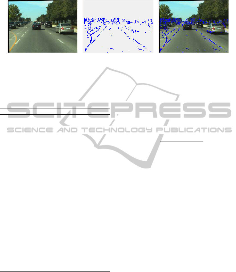
Figure 2: a) (left): Raw image b) (center): Low-level lane feature detection c) (right): Features depicted on the image.
while LD is its complement. Threshold τ
h
represents
the minimum gradient value required for a transition
from NL to LD. Constant O
h
is the minimum varia-
tion in height from the ground plane for a pixel to be
considered part of an obstacle. O
h
and τ
h
depend on
imagery and are experimentally determined.
Algorithm 1: Lane Feature Detection Algorithm.
G ← 1D Gaussian row smoothing of I with σ = 0.5
G ← horizontal gradient of G using 3-point central
differences
Remove the values corresponding to obstacles from
G using threshold O
h
State ←NL
F initialized to 0
for all rows i in I starting from the image bottom
do
L
max
← β −iα
Count ←0
for all column j in I do
if (G
i, j
> τ
h
∧(State = NL∨Count > L
max
))
then
State ←LD
end if
if (State = LD) ∧(G
i, j
< −τ
h
) then
for k = j −Count → j do
F
i,k
← 1
end for
State ←NL
Count ←0
end if
end for
end for
F ← 1D Gaussian row smoothing of I with σ = 0.5
The likelihood function (9) may be estimated us-
ing the extracted lane marking features F and the
sorted (from left to right) lane marking splines con-
tained in the visible spline buckets. The lane-marking
splines from the map are aligned with the direction of
the vehicle by a rotation and then projected on the im-
age plane so as to find a best fit with the detected lane
marking features. Assuming that the Z axis of the 3D
reference frame of the front stereo system of the vehi-
cle makes an angle θ with the Y axis of the 2D refer-
ence frame of the lane map, a spline point Q = (X,Y)
in the coordinates of the lane map is rotated according
to:
X
r
Z
r
=
cos(θ) sin(θ)
cos(θ) −sin(θ)
X
Y
(10)
With the ground plane equation, we estimate the tilt-
corrected height coordinate in the reference frame of
the stereo system as:
Y
r
=
d −aX
r
−Z
r
(c+ δλ)
b
(11)
where Q
r
= (X
r
,Y
r
,Z
r
) is the 3D spline point ex-
pressed in the reference frame of the stereo system.
The projection of Q
r
onto the stereo imaging plane
is performed by applying the classical projection ma-
trix P obtained for the calibration process of the stereo
system:
w
u
v
1
= P
X
r
Y
r
Z
r
1
(12)
where w is a scaling factor due to the use of homoge-
neous coordinates.
With the lane feature image F and the projected,
visible lane-marking splines, the likelihood function
becomes
L (z|x) =
∑
(i, j)∈S
F(i, j) (13)
where S is the set of all projected points of the lane-
marking splines.
3.3 Particle Filtering
With the likelihood function, we need to estimate the
parameters x of the fit as:
x = argmaxL (z|x)
x
(14)
Solving this optimization problem is not easily
achievable by regular hill-climbing methods due to
Map-basedLaneandObstacle-freeAreaDetection
527
the non-concavity of the function. Since the search
space is large, an exhaustive search is prohibitively
expensive while the probability of finding the global
maximum remains low (Talbi and Muntean, 1993).
A particle swarm method may be more appro-
priate. The particle swarm lane detection algorithm
by Zhou (Zhou et al., 2005) is a single image frame
method, which we adapt here as a particle filter work-
ing on a sequence of frames
2
. Our approach consists
of generating a set of uniformly distributed particles,
each representing a set of possible values for parame-
ters x = δx,δθ,δλ. The likelihood of each particle is
estimated with (14).
At each iteration, each particle is replaced with
a number of newly generated, Gaussian position-
disturbed particles. The number of generated particles
is proportionalto the likelihood of the particle they re-
place. Their likelihood are estimated again with (14)
and normalized. This ensures that the stronger parti-
cles generate more particles in their vicinity than the
weaker ones. Particles with normalized likelihoods
lower than a certain threshold are removed and, if the
number of particles becomes less than a threshold, the
process repeats.
These iterations eventually lead to groups of par-
ticles concentrated at the most likely answers in the
search space and the particle with the maximum like-
lihood is chosen as the solution. In addition, keeping
the particles over time makes the particle filter to act
as a tracker for the lane detection mechanism.
4 OBSTACLE DETECTION
With a set of detected lanes represented by projected
splines, the stereo depth map can be used to lo-
cate obstacles within each detected lane. The in-
puts to the obstacle-free detection algorithm are the
stereo disparity map I
d
, the classical projection and
re-projection matrices P and D, the ground plane pa-
rameters a, b, c, d, and δλ, and the projected lane-
marking splines. The output consists of the distance
from the vehicle to first obstacle (if present) for each
lane. The algorithm uses constant O
h
as previously
defined, and threshold O
t
which is the minimum ratio
of obstacle pixels to all pixels across a lane, for each
row in the image.
The first stage of the algorithm consists of detect-
2
PSO is a population-based stochastic optimization
method first proposed by Eberhart and Kennedy (Kennedy
and Eberhart, 1995).
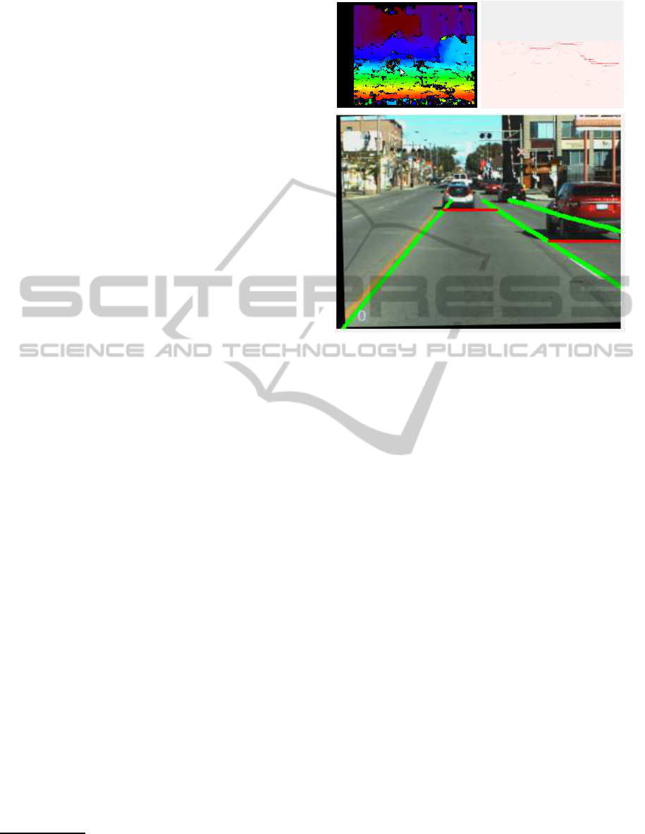
Figure 3: a) (top-left): Color-coded stereo depth map b)
(top-right): Accumulated projected obstacle points c) (bot-
tom): Obstacle-free area detection.
ing pixels whose 3D positions computed as:
W
X
Y
Z
1
= D
u
v
d
1
(15)
are not lying on the ground plane. The distance of the
3D point from the ground plane is obtained as:
Dist = aX + bY + (c+ δλ)Z −d (16)
The algorithm keeps an obstacle map O the size of
the original image. The 3D coordinates of each pixel
whose height from the ground plane qualifies it as an
obstacle is projected onto the ground plane by setting
its Y coordinate according to (11), and then projected
onto the obstacle map O, using
w
u
′
v
′
1
= P
X
Y
g
Z
1
(17)
where the corresponding image location in O is incre-
mented by one.
The last stage of the algorithm consists of scan-
ning all rows of image O from the bottom. In each
row, between the boundaries of each lane which is not
yet blocked, the values of O at the positions across the
lane are summed up and divided by the total number
of pixels in that lane, forming a lane ratio γ. If this
VISAPP2014-InternationalConferenceonComputerVisionTheoryandApplications
528
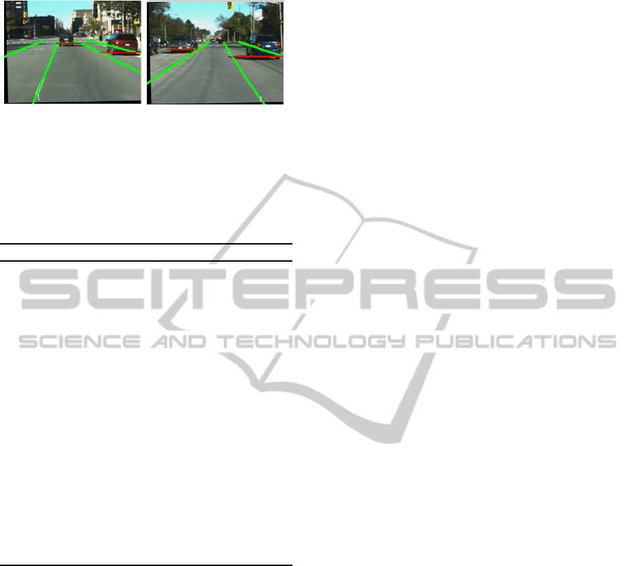
Figure 4: Examples of obstacle-free area detection re-
sults a) (left): Ongoing traffic within the detected lanes b)
(right): Incoming traffic outside of detected lanes.
ratio exceeds threshold O
t
, the lane is assumed to be
blocked by an obstacle at that row and the distance
of the obstacle is recorded for that lane. The formal
description of this algorithm is given in 2.
Algorithm 2: Obstacle-Free Zone Detection Algorithm.
O initialized to 0
for all O(u, v) do
Compute 3D coordinates of the point in the
stereo reference frame using I
d
and (15)
Dist ← aX + bY + (c+ δλ)Z−d
if Dist > O
t
then
Y
g
← (d −aX −(c+ δλ)Z)/b
Compute (u
′
,v
′
) using (17)
O
(u
′
,v
′
)
← O
(u
′
,v
′
)
+ 1
end if
end for
for all rows i in O do
for all lanes do
if lane ratio γ > O
t
and lane still open then
Output the lane as a blocked lane at corre-
sponding distance
end if
end for
end for
5 EXPERIMENTAL RESULTS
We applied this approach to a set of sequences
recorded form an instrumented experimental vehicle
(Beauchemin et al., 2010). The implementation of
the technique executes at 15Hz, including the stereo
depth computation, ground plane detection, particle
filtering for lane detection, and obstacle-free area es-
timation. Thirty initial particlesfor the particle swarm
were used, and the stereo image size was 320 by 240
pixels.
The experiments subjectively demonstrate that the
algorithm is robust to occlusion and partially worn-off
or occluded lane markers and various urban artifacts.
As observed, our technique remains stable, even for
some frames without any evidence of lane markers,
which is very difficult for most of the existing lane
detection approaches. Even in the presence of signif-
icant lane marker occlusions, our approach still prop-
erly detects lanes.
To our knowledge, vehicular imagery with anno-
tated lanes and precise GPS data for the recording ve-
hicle do not exist at this time, preventing an empirical
evaluation of our algorithms. Among our short-term
objectives is to produce such annotated sequences for
comparative purposes. However, problems such as
precisely determining the GPS position of the experi-
mental vehicle for such sequences remain elusive and
need to be surmounted.
One may argue that the requirement for GPS-
addressable, lane-annotated maps limits the areas in
which this approach may be used, which is correct.
However, we believe this approach can be used in
most driving situations, so long as lane-annotated
maps are automatically generated and made avail-
able to instrumented vehicles. Additionally, the con-
fidence measure obtained from thresholding the like-
lihood function may be used to assess the reliability
of detected lanes.
6 CONCLUSIONS
We proposed a map-based lane detection and
obstacle-free area detection using lane-annotated
maps, particle filtering, and stereo depth maps. Our
main contribution consists of our lane model obtained
from lane-annotated maps, allowing us to represent
irregular, opening, and closing lanes that are often ig-
nored in the current literature. Ironically, these types
of lanes are crucially important for iADAS as they
occur in critical areas such as intersections and merg-
ing and turning areas which constitute perilous zones.
Our approach uses a robust model that does not en-
tirely depend on an on-board imaging system which
may at times lead astray by the presence of occluding
obstacles and worn-off lane markers.
REFERENCES
Beauchemin, S., Bauer, M., Laurendeau, D., Kowsari, T.,
Cho, J., Hunter, M., and McCarthy, O. (2010). Road-
lab: An in-vehicle laboratory for developing cognitive
cars. In 23rd International Conference on Computer
Applications in Industry and Engineering, pages 7–
12.
Borkar, A., Hayes, M., Smith, M. T., and Pankanti, S.
(2009). A layered approach to robust lane detection
at night. In IEEE Workshop on Computational Intel-
Map-basedLaneandObstacle-freeAreaDetection
529

ligence in Vehicles and Vehicular Systems, pages 51–
57.
Catmull, E. and Rom, R. (1974). A class of local inter-
polating splines. Computer-Aided Geometric Design,
Academic Press, New York, pages 317–326.
Cheng, H.-Y., Jeng, B.-S., Tseng, P.-T., and Fan, K.-C.
(2006). Lane detection with moving vehicles in the
traffic scenes. IEEE Transactions on Intelligent Trans-
portation Systems, 7(4):571–582.
Hillel, A. B., Lerner, R., Levi, D., and Raz, G. (2012). Re-
cent progress in road and lane detection: a survey. Ma-
chine Vision and Applications, pages 1–19.
Huang, A. S., Moore, D., Antone, M., Olson, E., and Teller,
S. (2009). Finding multiple lanes in urban road net-
works with vision and lidar. Autonomous Robots,
26(2):103–122.
Jiang, Y., Gao, F., and Xu, G. (2010). Computer vision-
based multiple-lane detection on straight road and in
a curve. In IEEE International Conference on Image
Analysis and Signal Processing, pages 114–117.
Kennedy, J. and Eberhart, R. (1995). Particle swarm opti-
mization. In IEEE International Conference on Neu-
ral Networks, volume 4, pages 1942–1948.
Kim, Z. (2008). Robust lane detection and tracking in chal-
lenging scenarios. IEEE Transactions on Intelligent
Transportation Systems, 9(1):16–26.
McCall, J. C. and Trivedi, M. M. (2006). Video-based lane
estimation and tracking for driver assistance: survey,
system, and evaluation. IEEE Transactions on Intelli-
gent Transportation Systems, 7(1):20–37.
Narita, Y., Katahara, S., and Aoki, M. (2003). Lateral posi-
tion detection using side looking line sensor cameras.
In Intelligent Vehicles Symposium, pages 271–275.
Nieto, M., Salgado, L., Jaureguizar, F., and Arr´ospide, J.
(2008). Robust multiple lane road modeling based on
perspective analysis. In 15th IEEE International Con-
ference on Image Processing, pages 2396–2399.
Pomerleau, D. (1995). Ralph: Rapidly adapting lateral posi-
tion handler. In Proc. Intelligent Vehicles Symposium,
pages 506–511.
Rasmussen, C. and Korah, T. (2005). On-vehicle and aerial
texture analysis for vision-based desert road follow-
ing. In IEEE Conference on Computer Vision and Pat-
tern Recognition, pages 66–66.
Samadzadegan, F., Sarafraz, A., and Tabibi, M. (2006). Au-
tomatic lane detection in image sequences for vision-
based navigation purposes. In Proceedings of the IS-
PRS Commission, 5th Symposium on Image Engineer-
ing and Vision Metrology.
Sawano, H. and Okada, M. (2006). A road extraction
method by an active contour model with inertia and
differential features. IEICE Transactions on Informa-
tion and Systems, 89(7):2257–2267.
Talbi, E.-G. and Muntean, T. (1993). Hill-climbing, sim-
ulated annealing and genetic algorithms: a compara-
tive study and application to the mapping problem. In
IEEE Proceedings of the 26th International Confer-
ence on System Sciences, volume 2, pages 565–573.
Watt, A. and Watt, M. (1991). Advanced rendering and
animation techniques: Theory and practice. Reading,
MA.
Wu, S.-J., Chiang, H.-H., Perng, J.-W., Chen, C.-J., Wu, B.-
F., and Lee, T.-T. (2008). The heterogeneous systems
integration design and implementation for lane keep-
ing on a vehicle. IEEE Transactions on Intelligent
Transportation Systems, 9(2):246–263.
Zhou, Y., Hu, X., and Ye, Q. (2005). A robust lane de-
tection approach based on map estimate and particle
swarm optimization. In Computational Intelligence
and Security, pages 804–811. Springer.
VISAPP2014-InternationalConferenceonComputerVisionTheoryandApplications
530
