Local Analysis of Confidence Measures for Optical Flow Quality
Evaluation
Patricia M
´
arquez-Valle
1
, Debora Gil
1
, Rudolf Mester
2
and Aura Hern
`
andez-Sabat
´
e
1
1
Computer Vision Center, Universitat Aut
`
onoma de Barcelona, Edifici O - Campus UAB, Bellaterra, Barcelona, Spain
2
Visual Sensorics and Information Processing Lab, J. W. Goethe Universit
¨
at, Frankfurt, Germany
Keywords:
Optical Flow, Confidence Measure, Performance Evaluation.
Abstract:
Optical Flow (OF) techniques facing the complexity of real sequences have been developed in the last years.
Even using the most appropriate technique for our specific problem, at some points the output flow might fail
to achieve the minimum error required for the system. Confidence measures computed from either input data
or OF output should discard those points where OF is not accurate enough for its further use. It follows that
evaluating the capabilities of a confidence measure for bounding OF error is as important as the definition
itself. In this paper we analyze different confidence measures and point out their advantages and limitations
for their use in real world settings. We also explore the agreement with current tools for their evaluation of
confidence measures performance.
1 INTRODUCTION
Optical flow is a powerful tool for 3D reconstructions,
pedestrian detection, surveillance systems, medical
imaging assessment, etc. Its computation in real-
world is a challenging task due to, among others, il-
lumination changes, noise or textureless regions (Bar-
ron et al., 1994). Most of current research focus their
efforts on defining new algorithms in order to reduce
the impact of OF inaccuracies produced by the above
artifacts. Current algorithms are tested and compared
to each other by means of databases with ground truth
(McCane et al., 2001; Baker et al., 2011; Liu et al.,
2008; Butler et al., 2012). However, most of the avail-
able scenarios of databases are poorly assorted (ur-
ban, small objects, etc.) with only changes on illumi-
nation and object motion. Another concern is that the
number of frames available for each sequence may be
small. Even though recent databases for optical flow
evaluation are more realistic, they are far from mod-
eling the complexity and variability of real sequences
(Butler et al., 2012). Consequently, even if a method
performs properly on such databases, its performance
could fail in real-world conditions.
In order to use optical flow in a confident deci-
sion support system, a mechanism to detect sequence
pixels that have high error in their computations is of
prime importance. In this context, Confidence Mea-
sures (CM) should be an indicator of the accuracy of
the output of an optical flow algorithm. It should be
noted that a confidence measure can provide at most
an upper bound of OF error at each pixel, not its real
value (according to numerical error analysis (Cheney
and Kincaid, 2008)). This implies that high values of
the confidence measure should ensure a low OF error,
while for low CM values errors could take any value.
Points that have high error and high value of the con-
fidence measure are unpredictable points which CM
can not discard and, thus, should be the least possi-
ble.
Evaluating the quality of a confidence measure, as
well as analyzing the origin of unpredictable points,
are issues as important as the definition of a con-
fidence measure itself. Up to our knowledge, the
only ways of assessing CM performance are the Spar-
sification Plots, SP, introduced in (Bruhn and We-
ickert, 2006) and Error Prediction Plots, EPP, intro-
duced in (M
´
arquez-Valle et al., 2012). On the one
hand, SP show the average OF error across CM per-
centiles. Sparsification plot is the most widespread
tool for studying the general behavior of confidence
measures allowing an overall comparison across mea-
sures. However, being based on error global statistics,
they are not well suited for detecting unpredictable
points. On the other hand, EPP partially overcome
such limitation and, by definition, they are better de-
signed to detect artifacts in CM-OF error scatter plots.
A main concern is that, none of the existing CM eval-
450
Márquez-Valle P., Gil D., Mester R. and Hernàndez-Sabaté A..
Local Analysis of Confidence Measures for Optical Flow Quality Evaluation.
DOI: 10.5220/0004663304500457
In Proceedings of the 9th International Conference on Computer Vision Theory and Applications (VISAPP-2014), pages 450-457
ISBN: 978-989-758-009-3
Copyright
c
 2014 SCITEPRESS (Science and Technology Publications, Lda.)

uations explore the local pixel-wise behavior of con-
fidence measures and the sources of unpredictable
points.
In this paper we propose exploring the sources
of unpredictable points for existing types of CM. We
present two main contributions. First, we analyze the
local image intensity and OF patterns in order to de-
termine the sources of CM failing cases. Second, we
explore whether CM error bounding capabilities are
reflected by current ways of evaluating CM perfor-
mance. In this manner, this paper settles the ground
for further improvement of confidence measures and
their evaluation.
The paper is organized as follows. Section 2
briefly describes the state of the art confidence mea-
sures and performance evaluation methods. Section
3 analyzes, through some examples, the capabilities
of confidence measures for bounding the error. There
is also an analysis of the capabilities of SP and EPP
to detect when the confidence measures are able to
bound the error. Finally, the discussions, conclusions
and future work are given in section 4.
2 STATE OF THE ART
This section is devoted to briefly describe how most
of optical flow techniques compute the flow field, and
also identify the different types of errors they can pro-
duce. As well, in this section, the state of the art con-
fidence measures and current frameworks that allow
to evaluate CM’s performance are described.
Most of current optical flow techniques compute
the flow field by minimizing a variational (Horn and
Schunck, 1981) that combines a data-term and a
smoothness-term:
E(u,v) =
Z
D(u,v, ∇I)
| {z }
Data Term
+α S(∇u,∇v)
| {z }
Smoothness Term
dx dy (1)
for I(x,y,t) denoting the image sequence, (u,v) the
flow field and ∇ the sequence gradient. The data-
term is usually based on the optical flow constraint,
I
x
u + I
y
v + I
t
= 0, and the smoothness-term models
the general properties of the flow field. The minimum
of (1) is computed by solving the associated Euler-
Lagrange equations.
Errors of the resulting flow can be split into two
main categories (M
´
arquez-Valle et al., 2012): errors
in OF model and numerical errors:
Model Errors. The formulation of optical flow relies
on some assumptions on the input data and flow mo-
tion. Brightness constancy constraint, or some regu-
larity of the motion flow (Horn and Schunck, 1981;
Lucas and Kanade, 1981) are common assumptions
of optical flow algorithms. In case these assumptions
are not satisfied (brightness changes for instance) the
output vector is less reliable and might fail to properly
model sequence motion.
Numerical Errors. The input data for OF computa-
tion might contain errors that are propagated through
the computations, and, thus, introduce errors in the
output flow. The impact of input errors propagation,
depends on the numerical stability of optical flow
formulation and can be explored by means of numeric
analysis tools (Cheney and Kincaid, 2008).
2.1 Confidence Measures
The final purpose of a confidence measure should be
the detection of numerical errors and also, provide an
upper bound for the final error. Even though in the
literature there are several different confidence mea-
sures defined (Singh, 1990; Barron et al., 1994; Shi
and Tomasi, 1994; Bruhn and Weickert, 2006; Kon-
dermann et al., 2008; Sundaram et al., 2010; Kybic
and Nieuwenhuis, 2011; Gehrig and Scharwachter,
2011; M
´
arquez-Valle et al., 2012; Mac Aodha et al.,
2013; Senst et al., 2012), we only explore four of the
most representative ones:
Energy. Under the (sensible) assumption that all con-
strains have been taken into account in the definition
of the functional (1), the computed flow field will be
accurate in the measure that its local energy is low.
Under this consideration, the authors in (Bruhn and
Weickert, 2006) propose the following measure:
c
e
=
1
D(u,v, ∇I) + αS(∇u,∇v) + ε
2
(2)
where ε prevents dividing by zero. A main advantage
of c
e
is that it can be computed for any variational
scheme. A main concern is that c
e
only measures that
(u,v) minimizes equation (1) and, thus, fulfills the as-
sumptions made in the model. However, this does not
guarantee that (u,v) corresponds to the true flow field,
since defining the most appropriate optical flow con-
straints for a given application is still an open prob-
lem.
Statistical. In many applications, flow fields follow
similar local motion patterns. If such motion patterns
are learned a priori, then a classifier can be used to de-
fine a confidence measure. The measure introduced in
(Kondermann et al., 2008), which we note as c
s
, de-
rives natural motion statistics from sample data and
carries out a hypothesis test to obtain confidence val-
ues for the computed flow. The method depends only
LocalAnalysisofConfidenceMeasuresforOpticalFlowQualityEvaluation
451

on the resulting flow field and on the prior knowledge
learned from a database. The confidence measure as-
sesses the computed optical flow calculating the local
variability by means of the Mahalanobis distance be-
tween the computed vector and the distribution given
by the surrounding ones. Since the formulation is
not straight forward, we refer the reader to the paper
(Kondermann et al., 2008) for more details.
A main limitation of this measure is that unusual
motion patterns are not easy to learn and might re-
quire a huge database of different flow patterns to
train the model. This limits its use for sequences with
flow fields that are erratic or unpredictable. In addi-
tion, it only assesses if the flow field is coherent, but
not if the flow field corresponds to the sequence mo-
tion.
Bootstrap. The measure introduced in (Kybic and
Nieuwenhuis, 2011) aims at assessing the uncertainty
of the optical flow method with respect to the model
constraints. That is, they compute the variability of
the computed flow field using bootstrap by introduc-
ing numerical perturbations. If the variability is high,
the flow field is not reliable, whereas for low variabil-
ity, the computation is reliable. In order to have a
decreasing dependency with the accuracy is rewritten
follows:
c
b
=
1
ψ
bootg
+ ε
2
, ψ
bootg
=
q
σ
2
u
+ σ
2
v
(3)
where ε prevents dividing by zero, and σ
u
and σ
v
are
the variances of the flow field (u,v) after the boostrap
computation. For more details of ψ
bootg
defined in
(Kybic and Nieuwenhuis, 2011), we refer the reader
to eq. (15) of that paper. Like c
e
, this one also as-
sesses the consistency of the model assumptions, but
also assesses the errors produced by numerical stabil-
ity of the method. However, c
b
requires to be rede-
fined for each optical flow technique and it is compu-
tationally costly.
Image Local Structure. Some confidence measures
are defined by means of the structure tensor of the
image, and thus, they use information about the lo-
cal structure of the image. There are several mea-
sures derived from the structure tensor: determinant,
trace (Barron et al., 1994), lowest eigenvalue (Shi and
Tomasi, 1994) among others. These measures only
detect errors produced due to the image, that is, tex-
tureless regions, noise, etc. However, they do not con-
sider the errors produced by during the computations.
An improved measure that uses the structure tensor,
considers the condition number of the structure ten-
sor matrix (M
´
arquez-Valle et al., 2012):
c
k
=
λ
min
λ
max
(4)
for λ
min
and λmax the minimum and maximum
eigenvalues of the structure tensor at a given pixel
location. This measure, not only assesses the capabil-
ities of the image to compute the flow field, but also
assesses the numerical stability of the computation
for Lucas-Kanade based schemes (Lucas and Kanade,
1981; Bruhn et al., 2005).
2.2 Performance Evaluation of
Confidence Measures
Scatter plots showing CM against OF errors are a
good tool to assess the relation between both quan-
tities, as illustrated in fig.1. A perfect CM should pro-
duce decreasing profiles, like the one shown in middle
plots. Points inside the red square in the first scatter
correspond to points which error is not bounded by
the confidence measure. Given that those points could
introduce a significant error in a decision support sys-
tem using OF, evaluation of the confidence measure
should detect the scope of such unpredictable points.
The most extended way to represent the perfor-
mance of a confidence measure is by means of the
Sparsification Plots, SP (Bruhn and Weickert, 2006).
Such plots are given by the remaining mean error
for fractions of removed flow vector having increas-
ing confidence measure values. That is, the confi-
dence measure is increasingly sorted, then, from 0%
to 100%, a percentage of flow vectors is removed and
the average error of the remaining ones is computed.
The arrows of the scatter plots shown in the first row
of fig.1 illustrate the computation of the SP shown in
the last plot. Under the assumption that higher values
of the confidence measure are associated to lower op-
tical flow errors, the sparsification plots should have
decreasing profiles. An increase in their values for
the higher removed fractions indicates artifacts in the
decreasing dependency possibly due to a high error.
However, the inverse does not always hold and ran-
dom uniform dependencies could produce sensible
plots. This is the case of the first representative se-
quence shown in fig. 1. Even if the dependency
shown in the scatter plot is worse in the first sequence,
its SP (blue line in the last plot of fig1) indicates a bet-
ter performance for higher fractions.
Another way to represent the performance of con-
fidence measures are the Error Prediction Plots, EPP
(M
´
arquez-Valle et al., 2012). Such plots provide a
global vision of the capability of confidence measures
to discard high errors. The error prediction plots are
computed by means of the conditional probabilities
across the diagonal of the CM-OF error scatter plots.
P
C
(τ
EE
,τ
CM
) := P(EE ≥ τ
EE
|CM ≥ τ
CM
) (5)
VISAPP2014-InternationalConferenceonComputerVisionTheoryandApplications
452

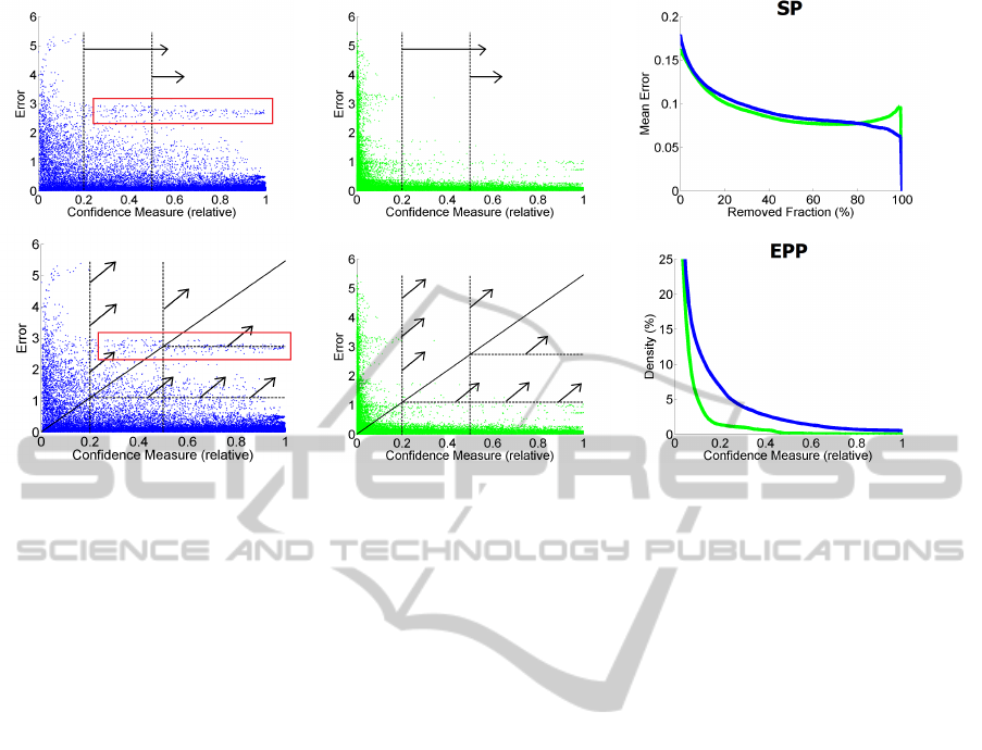
Figure 1: Existing evaluations of Confidence Measures: first row, SP and second row, EPP. First and second columns show
Scatter plots of a confidence measure versus OF errors (for two different cases colored in blue and green). Red squares on the
first column denote outliers. The black lines and arrows show how the SP and EPP are computed respectively. SP and EPP of
both measures are shown on third column.
for P
C
(τ
EE
,τ
CM
) the probability of having an error
EE above τ
EE
provided that CM is above τ
CM
. Tak-
ing into account that the condition CM ≥ τ
c
corre-
sponds to a vertical line and EE ≥ τ
EE
to an hori-
zontal one, the conditional probability is given by the
fraction of points lying on the superior quadrant de-
fined by the former lines. The EPP are defined as the
plot given by (CM, P
C
(EE
max
·CM/CM
max
,CM)), for
EE
max
the maximum error allowed by the application
and CM
max
, CM maximum value. The scatter plots
in the second row of fig.1 illustrate the computation
of (5) for two representative cases. Arrows indicate
the points that are considered for the computation of
conditional probabilities. Unlike the SP shown in the
first row of fig.1, we observe that EPP is worse for the
non-decreasing case.
3 ANALYSIS OF CONFIDENCE
MEASURES
The main purpose of this section is to help to bet-
ter understand a confidence measure behavior and its
weak and strong points for bounding OF error. In par-
ticular we will address two main issues: first, we are
interested in finding the local conditions (both in ap-
pearance and motion) that a sequence should fulfill
in order that a CM succeeds in bounding the error of
a particular OF method. Second, we will assess, the
capability of SP and EPP for detecting those points
where the confidence measure is not able to bound
the error.
In order to explore CM bounding capabilities we
locally analyze the behavior of confidence measures
for a selected sample of sequence patches. These
patches cover the main appearance and motion fea-
tures that are prone to introduce an error in OF and
CM expected behaviors. In this context we have se-
lected patches violating:
• Data-term OF Constrain Assumptions. On
the one hand, the data term requires that there
is enough information in the image intensity to
compute the apparent 2D motion. On the other
hand, large displacements are against the first or-
der Taylor approximation given by the OF equa-
tion. Therefore, we have selected patches with
straight edges and textureless regions for their in-
tensity appearance as well as, patches of a large
displacement.
• Smoothness-term Regularity Assumptions. In-
dependent motions might interfere with the regu-
larity assumptions of the smoothness-term.
The maximum error used to compute EPP is
EE
max
= 2. We have considered the 4 confidence
measures described in section 2, c
k
, c
e
, c
b
and c
s
.
Results have been extracted from the Middlebury
database (Baker et al., 2011). This database contains
real-life and synthetic sequences with ground truth,
to show some examples we have used two frames of
the RubberWhale and the Urban sequences. Motion
LocalAnalysisofConfidenceMeasuresforOpticalFlowQualityEvaluation
453

has been computed using the Combined Local-Global
(CLG) scheme (Bruhn et al., 2005) as implemented in
(Liu, 2009)
1
. The error score is the End-Point Error
(EE) (Baker et al., 2011), it measures the difference
between computed flow field and ground truth.
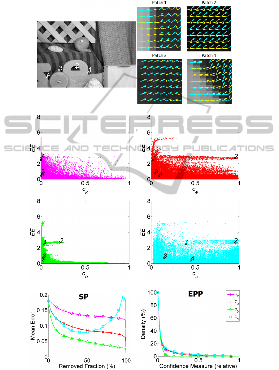
Figures 2 and 3 show our analysis for Rubber-
Whale and Urban3 sequences. Each figure shows
a sequence frame, four representative patches with
computed (yellow arrows) and ground truth (green ar-
rows) flows, CM-OF error scatter plots for each mea-
sure and SP, EPP plots. Each patch is of size 7 ×7 and
it is centered at the respective illustrative point shown
in the sequence frame and scatter plots.
Patches in fig.2 contain straight edges with inde-
pendent motions (patches 1 and 4), a textureless re-
gion with uniform motion (patch 2), and a texture-
less region with a slightly irregular motion (patch 3).
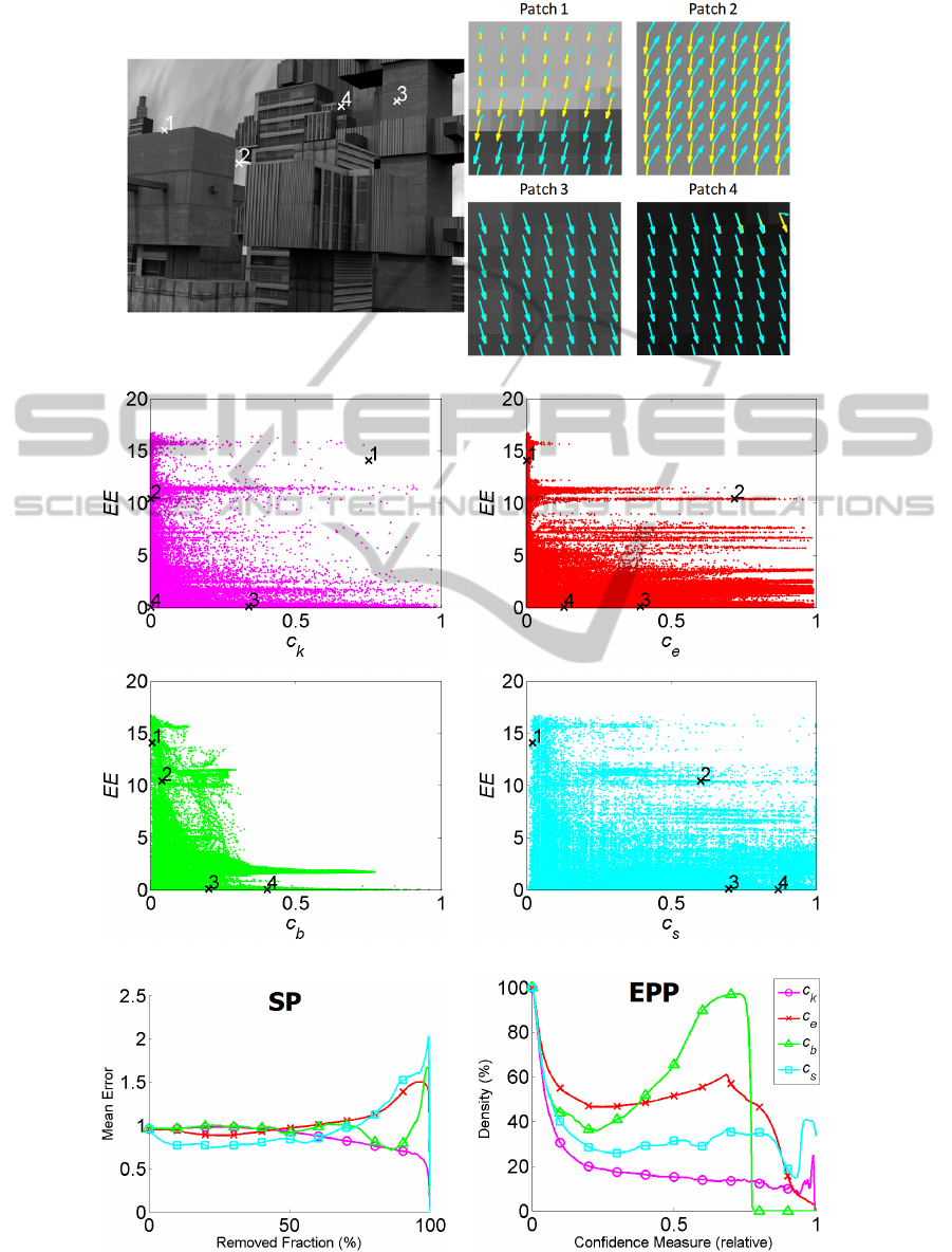
Patches in fig. 3 show a sloped border with a large
displacement of an object moving over a static back-
ground (patch 1), textureless regions with uniform
motions (patches 2 a 4) and a slightly textured region
with uniform motion (patch 3).
Concerning data term conditions, at straight edges
(patches 1, 4 in fig.2) and textureless regions (patch 2,
3 in fig.2 and 2,4 in fig.3) CLG can not solve the data
term. The lowest eigenvalue of the structure tensor
matrix is close to zero and this introduces large nu-
merical instability. We would like to note that in such
cases EE can take any value, ranging within 0 and 20
in our sequences. Numerical instability of the data
term is properly detected by low c
k
values. The data
term is numerically well-conditioned in the case of
sloped borders (patch 1 in fig.3) and textured regions
(patches 3 in fig.2 and 3). However, stable numerics
do not guarantee accurate OF, given that OF model
assumptions are also decisive for its accuracy. This is
the case of patch 1 in fig.3, which presents a high er-
ror due to the high displacement magnitude and, thus,
c
k
can not properly bound EE.
Regarding regularity conditions, the bounding ca-
pabilities of c
b
are more related to them assumptions
and, thus, it properly bounds EE at patches present-
ing independent moving objects (like patches 1, 4 in
fig.2 and patch 1 in fig.3). However, its capabilities
for error bounding decrease for patches with uniform
motion, given that c
b
is always high, but OF might
present a large error for textureless patches (patch 2
in fig.2). The measure based on energy minimization,
c
e
, is also associated to model assumptions, given that
at pixels which model regularity is not met, the func-
tional can not be properly minimized. This is the case
of patches with independent motions, like patches 1,
3, 4 in fig.2 and patch 1 in fig.3. Like c
b
, c
e
fails in
1
Available at http://people.csail.mit.edu/celiu/OpticalFlow/
the case of textureless regions with uniform motion
shown in patch 2 in fig.2 and patch 3 in fig.3.
Finally, the weakest measure for error bounding
purposes is c
s
, which scatters present the most uni-
form distribution of all. Such uniform distribution of
EE across c
s
values indicates that there is not a clear
relation between the measure and the error. In fact, it
only succeeds in bounding EE for patch 3 in fig.2 and
patch 1 in fig.3 that are the ones having a flow field
not regular around the central point. For the remain-
ing patches, OF is regular enough although this does
not necessarily imply it is accurate.
Concerning CM performance evaluation shown in
bottom plots, we note that the bounding artifacts de-
tected in c
e
profile in fig.2 are not properly reflected
by SP plots. On the contrary, c
k
decreasing profiles
do not always produce a best decreasing SP (fig.2).
This is due to only considering 1-dimensional statis-
tics over EE and not over the bimodal distribution
given by (CM,EE). By considering bimodal statis-
tics, EPP provides a better ordering of CM quality for
error bounding. In particular, it detects the groups of
unpredictable pixels introducing horizontal scatters in
CM-EE plots, like the ones present in c
b
and c
e
scatter
plots in fig.3.
4 DISCUSSIONS, CONCLUSIONS
AND FUTURE WORK
Evaluating the capabilities of a confidence measure
for optical flow error bounding is as important as its
definition. In this paper we have analyzed locally
the capabilities of confidence measures for bounding
the different types of OF error. We have also eval-
uated if current tools for confidence measure quality
assessment agree with confidence measures bounding
capabilities. Concerning the capabilities of existing
CMs for OF error bounding, the following interesting
points are derived from our analysis:
Energy (c
e
) confidence measure detects when the
functional is not properly minimized, and this usually
happens at borders. In addition, this confidence mea-
sure only detects points where the computation does
not correspond with the model assumptions, and thus
it detects points that satisfy the model assumptions
as reliable although they may not coincide with the
ground truth.
Statistical (c
s
) confidence measure detects if the
computed flow is not coherent, and, thus, points hav-
ing an OF either not regular or random. This implies
that a constant OF would always be reliable regardless
of its agreement with ground truth.
VISAPP2014-InternationalConferenceonComputerVisionTheoryandApplications
454

Illustrative Points
Scatter Plots
Performance Evaluation
Figure 2: RubberWhale sequence.
LocalAnalysisofConfidenceMeasuresforOpticalFlowQualityEvaluation
455

Illustrative Points
Scatter Plots
Performance Evaluation
Figure 3: Urban3 sequence.
VISAPP2014-InternationalConferenceonComputerVisionTheoryandApplications
456

Bootstrap (c
b
) confidence measure detects if the
model is unstable, that is, when small perturbations
in the input data produce high variations in the out-
put. Thus, it detects points that do not satisfy model
assumptions like edges of object following different
motions and textureless regions.
Image Local Structure (c
k
) confidence measure
detects those pixels the image structure is not appro-
priate to solve optical flow, like textureless regions,
and straight lines. However, textured regions may
contain a lot of noise disturbing computations and,
also, failing of OF assumptions is not considered.
We conclude that c
s
is not the best suited for
bounding OF error. Besides, c
k
, c
b
, c
e
are able to
bound a different kinds of error and, in fact, they pro-
vide complementary bounds.
Concerning existing methods for evaluation
of confidence measures, EPP better reflect non-
decreasing profiles between CM and OF error and,
thus, it is better suited for detecting CM unable to
bound errors for a significant amount of cases. How-
ever, none of the evaluation methods provides enough
information about confidence measures failing cases
and thus, further research is required.
As a future work it would be interesting to view
examples for patches with more than two motion
areas and illumination changes. Also use a larger
database. And finally, check the confidence measure
performances on different optical flow methods.
ACKNOWLEDGEMENTS
Work supported by the Spanish projects TIN2009-
13618, TIN2012-33116 and TRA2011-29454-C03-
01 and first author by FPI-MICINN BES-2010-
031102 program.
REFERENCES
Baker, S., Scharstein, D., Lewis, J., and et al. (2011). A
database and evaluation methodology for optical flow.
IJCV, 92(1):1–31.
Barron, J. L., Fleet, D. J., and Beauchemin, S. S. (1994).
Performance of optical flow techniques. IJCV,
12(1):43–77.
Bruhn, A. and Weickert, J. (2006). A confidence mea-
sure for variational optic flow methods. In Geometric
Properties for Incomplete Data, pages 283–298.
Bruhn, A., Weickert, J., and Schn
¨
orr, C. (2005). Lu-
cas/Kanade meets Horn/Schunck: Combining local
and global opticflow methods. IJCV, 61(2):221–231.
Butler, D. J., Wulff, J., Stanley, G. B., and Black, M. J.
(2012). A naturalistic open source movie for optical
flow evaluation. In ECCV, pages 611–625.
Cheney, W. and Kincaid, D. (2008). Numerical Mathemat-
ics and Computing, Sixth edition. Bob Pirtle, USA.
Gehrig, S. and Scharwachter, T. (2011). A real-time multi-
cue framework for determining optical flow confi-
dence. In ICCV Workshops, pages 1978–1985. IEEE.
Horn, B. and Schunck, B. (1981). Determining optical flow.
AI, 17:185–203.
Kondermann, C., Mester, R., and Garbe, C. S. (2008). A
statistical confidence measure for optical flows. In
ECCV, pages 290–301.
Kybic, J. and Nieuwenhuis, C. (2011). Bootstrap optical
flow confidence and uncertainty measure. Computer
Vision and Image Understanding, pages 1449–1462.
Liu, C. (2009). Beyond pixels: exploring new representa-
tions and applications for motionanalysis. PhD thesis,
Cambridge, MA, USA.
Liu, C., Freeman, W., Adelson, E., and Weiss, Y. (2008).
Human-assisted motion annotation. In CVPR.
Lucas, B. and Kanade, T. (1981). An iterative image regis-
tration technique with an application to stereovision.
In DARPA IU Workshop, pages 121–130.
Mac Aodha, O., Humayun, A., Pollefeys, M., and Brostow,
G. J. (2013). Learning a confidence measure for op-
tical flow. IEEE Trans. Pattern Anal. Mach. Intell.,
35(5):1107–1120.
M
´
arquez-Valle, P., Gil, D., and Hern
`
andez-Sabat
´
e, A.
(2012). A complete confidence framework for opti-
cal flow. In ECCV Workshops, volume 7584 of LNCS,
pages 124–133. Springer.
McCane, B., Novins, K., Crannitch, D., and Galvin, B.
(2001). On Benchmarking Optical Flow. Computer
Vision and Image Understanding, 84(1).
Senst, T., Eiselein, V., and Sikora, T. (2012). Robust local
optical flow for feature tracking. IEEE Trans. Circuits
Syst. Video Techn., 22(9):1377–1387.
Shi, J. and Tomasi, C. (1994). Good features to track. In
CVPR, pages 593–600.
Singh, A. (1990). An estimation-theoretic framework for
discontinuous flow fields. In ICCV, pages 168–177.
Sundaram, N., Brox, T., and Keutzer, K. (2010). Dense
point trajectories by gpu-accelerated large displace-
ment optical flow. In ECCV, pages 438–451.
LocalAnalysisofConfidenceMeasuresforOpticalFlowQualityEvaluation
457