
Contour based Split and Merge Segmentation and Pre-classification of
Zooplankton in Very Large Images
Enrico Gutzeit
1
, Christian Scheel
2
, Tim Dolereit
1
and Matthias Rust
3
1
Fraunhofer Institute for Computer Graphics Research IGD, Joachim-Jungius-Str. 11, 18059 Rostock, Germany
2
University of Rostock, Institute for Computer Science, Albert-Einstein-Str. 22, 18059 Rostock, Germany
3
Arivis AG, Kroepeliner Str. 54, 18055 Rostock, Germany
Keywords:
Segmentation, Contour, Split & Merge, Pre-classification, Shape Features, Zooplankton, Large Images.
Abstract:
Zooplankton is an important component in the water ecosystem and food chain. To understand the influence of
zooplankton on the ecosystem a data collection is necessary. In research the automatic image based recognition
of zooplankton is of growing interest. Several systems have been developed for zooplankton recognition on
low resolution images. For large images approaches are seldom. Images of this size easily exceed the main
memory of standard computers. Our novel automatic segmentation approach is able to handle these large
images. We developed a contour based Split & Merge approach for segmentation and, to reduce the non-
zooplankton segments, combine it with a pre-classification of the segments in reference to their shape. The
latter includes a detection of quasi round segments and a novel one for thin segments. Experimental results on
several large images show that we are able to handle them satisfactorily.
1 INTRODUCTION
Zooplankton and phytoplankton are a significant part
of the food chain of every aquatic ecosystem. Con-
sequently, they represent a fundamental parameter of
the ecosystem’s structure and act as an indicator of
its structural changes. The analysis can be done in
situ or in the laboratory with fixed and filtered plank-
ton samples. Expected results are the identification
of plankton in these samples and also their classifi-
cation into the appropriate species categories. The
usual approach starts with the deployment of plank-
ton nets followed by manual evaluation of the gath-
ered samples by a taxonomic expert. This is a labor
intensive and time consuming procedure which heav-
ily depends on rare expert knowledge. Hence, the au-
tomatic recognition of plankton is of growing interest
in biology. Many good reasons for automatic plank-
ton recognition are discussed by Gaston and O’Neill
(Gaston and O’Neill, 2004). A full solution for an
automatic or semi-automatic system should consist of
an image acquisition stage (laboratory or in situ) fol-
lowed by an image processing stage.
In this paper we concentrate on zooplankton sam-
ples acquired in a laboratory setup. We focus on the
segmentation of zooplankton and briefly describe the
image acquisition as well as the zooplankton recog-
nition. Our acquisition method is realized with low
cost equipment producing high resolution images in
size of about 60000×60000 pixels with a pixel size
of about 0.4 µm. Images of this size easily exceed
the main memory of standard computers. Our follow-
ing novel automatic segmentation approach is able to
handle these large images. It comprises an adjusted
segmentation of all the objects in the image and a pre-
classification to eliminate non-zooplankton segments.
The paper is organized as follows. Section 2
presents related work and in section 3 the problems
to solve are discussed. Our approach to image acqui-
sition and image processing is explained in section 4.
In section 5 we discuss our results and we finish with
conclusions and future works in section 6.
2 RELATED WORK
The recognition and quantification process can be
supported by different techniques. The approaches of
(Sheldon and Parsons, 1967), (Fawell, 1976), (Her-
man and Dauphinee, 1980), for instance, do not in-
volve image processing methods, but electronic, col-
orimetric or ultrasonic measuring methods. Image
processing is a powerful tool for automatic recog-
nition and classification of zooplankton. A typi-
cal analysis pipeline starts with the image acquisi-
tion and consists of segmentation, feature extraction,
training and classification stages. Some first exam-
417
Gutzeit E., Scheel C., Dolereit T. and Rust M..
Contour based Split and Merge Segmentation and Pre-classification of Zooplankton in Very Large Images.
DOI: 10.5220/0004648604170424
In Proceedings of the 9th International Conference on Computer Vision Theory and Applications (VISAPP-2014), pages 417-424
ISBN: 978-989-758-003-1
Copyright
c
2014 SCITEPRESS (Science and Technology Publications, Lda.)
ples are the works of (Katsinis, 1979) or (Jeffries
et al., 1984). Common shape features for classifica-
tion are extracted from the threshold-segmented im-
ages of low resolution (256×256 px). The images in
(Chehdi et al., 1986), taken through a microscope, are
already slightly bigger (512×512 px). Our work con-
centrates on images many times larger and requires
advanced methods for automatic segmentation.
More recent and also technically more mature ap-
proaches mostly contain a special imaging device in
combination with a specific image processing system.
Imaging devices can be specialized to work either in
situ or in a laboratory. In situ devices are able to
image flowing particles in a volume of water over
time. They are mostly constructed as mooring buoy,
towed body or as an installation on a ROV or AUV.
A first example for an in situ device is the Video
Plankton Recorder (VPR) (Davis et al., 1992). An
identification Software, the Visual Plankton, to rec-
ognize plankton in images taken by the VPR is de-
scribed in (Davis et al., 2005). The image acqui-
sition is adjustable between a resolution of 10 µm
and 300 µm per pixel. The segmentation is done af-
ter binarization and regions of interest (ROIs) are ex-
tracted. Another system is the Shadowed Image Par-
ticle Profiling Evaluation Recorder (SIPPER) (Sam-
son et al., 2001) with the Plankton Image Classifica-
tion and Extraction Software (P.I.C.E.S.) (Luo et al.,
2004). Binary images with a pixel resolution of 50
µm are produced and hence, a segmentation is al-
ready given. The Underwater Vision Profiler (UVP)
(Picheral et al., 2010) is suited for real-time, in situ
particle counting, sizing and zooplankton detection
(Website, 2013b). This is done by integrating a dedi-
cated software within an intelligent camera, which is
able to remove a background image. The pixel reso-
lution of the images amounts to 174 µm. Further sys-
tems are the HAB-Buoy (Culverhouse et al., 2006)
coupled to the Dinoflagellate Categorisation by Arti-
ficial Neural Network (DiCANN) software (Toth and
Culverhouse, 1999), the In Situ Ichtyoplankton Imag-
ing System (ISIIS) (Tsechpenakis et al., 2007; Tsech-
penakis et al., 2008), the ImagingFlowCytobot (Ol-
son and Sosik, 2007) and CytoBuoy (Dubelaar and
Jonker, 2000).
In a laboratory setup, like our scenario, water sam-
ples can be prepared and analyzed. The commer-
cial system Flow Cytometer And Microscope (Flow-
CAM) (Sieracki et al., 1998) is equipped with the
software Visual Spreadsheet (Website, 2013a). The
software is able to extract sample particle sizes of 2
µm to 2 mm after segmentation and stores the ROIs.
No details on the process are given. The system most
comparable to ours is ZooScan (Gorsky and Gros-
jean, 2003) with the software Zooprocess and Plank-
ton Identifier (Website, 2013c). Zooscan is a water-
proof scanner with a maximal resolution of 2400dpi
resulting in a pixel size of 10.6 µm. On Zooscan’s
website is stated: ”if all available image dimensions
can be acquired, there is still some limitation for the
largest images processing. We are working on new
macros that will overcome these limitations soon”.
In Zooprocess a background image is substracted to
segment and extract individual objects. Zooprocess
and Plankton Identifier are also able to process im-
ages from UVP.
Existing systems are not able to produce or handle
large images as required in our scenario. Particularly,
the published post-processing and segmentation algo-
rithms require the images to fit into the computer’s
main memory.
3 DISCUSSION OF PROBLEMS
In our scenario, zooplankton species inside a counting
chamber with water (diameter 25 mm) have to be rec-
ognized. Images of the chamber are taken stepwise
by a microscope camera.
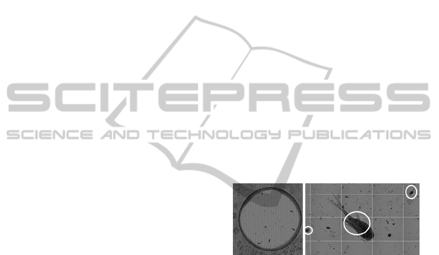
Figure 1: The counting chamber (left) and a part of it (right)
with small and large species are shown. The stitched tiles
are illustrated through lines and species with circles.
The images (tiles) are stitched together to a large
image (approx. 60000×60000 px), which is illus-
trated in figure 1. The zooplankton is located only
inside the counting chamber. Hence, it is helpful for
further processing to detect the contour of this cham-
ber. For recognition, a segmentation of the zooplank-
ton is needed. The following problems must be solved
to segment the zooplankton. Different zooplankton
species can vary in size and in positioning. Some
species can overlap multiple tiles due to a position
on the border and large species can be even bigger
than a single tile. On the contrary, small species can
be similar in size of an unimportant particle (non-
zooplankton). A further problem is the size of the
image, which is too big for processing at once. Also,
there are visible side effects after the stitching process
due to illumination variances that lead to high gradi-
ents at the borders of the acquired tiles.
VISAPP2014-InternationalConferenceonComputerVisionTheoryandApplications
418
To overcome the problems we developed a con-
tour based Split & Merge approach for segmentation.
We do not split the image in homogenous regions
and merge similar regions like in (Kelkar and Gupta,
2008). In our approach we split the image in regular
tiles and merge the segmented contours in an itera-
tive way. Furthermore, to reduce the non-zooplankton
segments we implemented a pre-classification of the
segments in reference to their shape. Our novel seg-
mentation and pre-classification approach will be de-
scribed in following section.
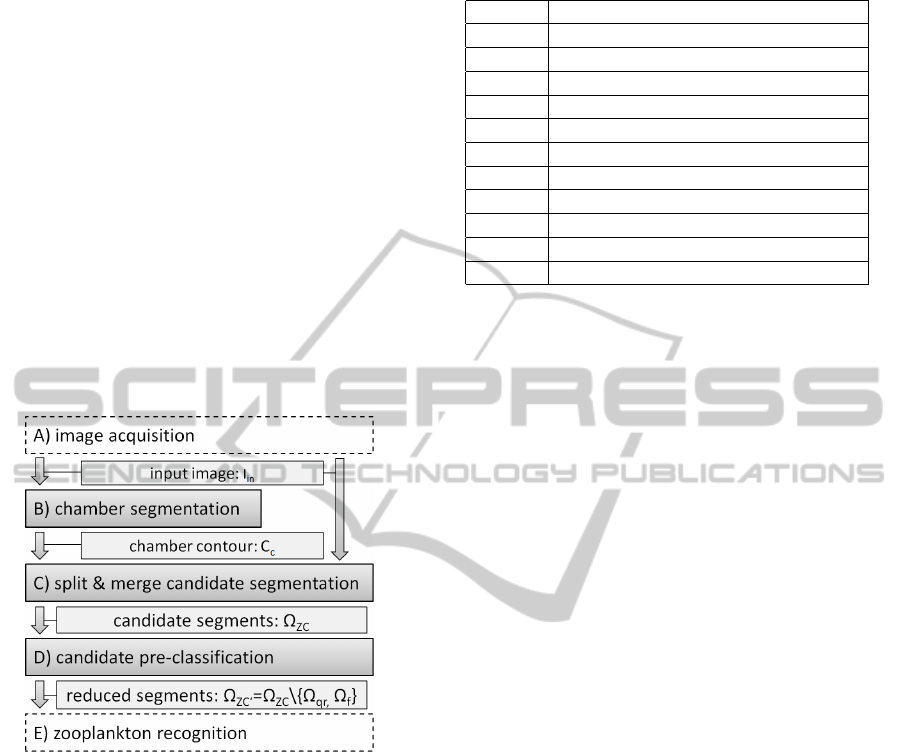
4 OUR APPROACH
Our approach to segment and pre-classify zooplank-
ton is divided into five steps, which is illustrated in
figure 2.
Figure 2: Our segmentation and pre-classification proce-
dure for very large images.
In step A the images are acquired with an in-
verted dissected light microscope setup. The im-
ages are stitched together and post processed into a
large grayscale input image. Thereafter, in step B,
the contour of the counting chamber is detected to
reduce the region to be processed in the following
steps. The region inside the chamber is segmented
in step C with a Split & Merge approach. As result
we get segments representing zooplankton and non-
zooplankton of different kinds. In step D we execute
the pre-classification to simplify the recognition pro-
cess. Thereby, we can reduce the non-zooplankton
set in our scenario. Finally, a zooplankton recogni-
tion with a support vector machine (SVM) is done in
step E. In this paper we set the focus on step B, C
and D. An overview of the main notations used in this
paper is given in table 1.
Table 1: Main notation used in this paper.
I
in
large grayscale input image
C, P contour and point in general
C
c
the counting chamber contour
C
zc
a zooplankton candidate contour
C
Ql
a contour in a quadtree leaf
C
∗
,C
+
a complete and incomplete contour
Q, Q
l
quadtree, quadtree leaf
Q
rb
right and bottom quadtree neighbor
P
s
, P
e
start and end contour merging point
Ω
ZC
zooplankton candidate segment set
Ω
qr
, Ω
t
set of quasi round and thin segments
Ω
ZC
0
reduced set of zooplankton candidate
4.1 Image Acquisition
We used counting chambers with a glass bottom
(Utermoehl, Kolkwitz) and an inverted dissected light
microscope setup (Olympus IX50). Due to the re-
quired resolution and the thickness of the sample we
added a motorized xyz-stage (Maerzhaeuser) to sup-
port tiled acquisition (xy) in multiple focus planes (z).
Sufficient results were achieved with a 10× magni-
fication lens and a total number of 5 focus planes,
which leads to a data size in the gigabyte range.
The acquisition is controlled by the imaging software
arivis Browser with an acquisition module that is con-
nected to the microscope components and allows the
definition of the required acquisition strategies and
parameters. The single tiles are acquired as RGB
images with a configurable overlap for compensating
small variations in the motor stage positioning. Af-
ter acquiring the single images an automated stitching
and intensity compensation are performed to create a
large plane from the single tiles. Color information
is not utilized for subsequent steps, so all planes are
converted to one greyscale plane.To further reduce the
amount of data, an edge blending algorithm was ap-
plied that creates one merged image from the single
focus planes by selecting pixels with the highest con-
trast.
4.2 Chamber Segmentation
Zooplankton is positioned only inside the counting
chamber (see figure 1). For this reason, the detection
of the chamber contour C
c
is required. We have scaled
the large image to a width of 2048 pixel. The follow-
ing methods were implemented and tested for their
ability to extract the contour of the counting chamber
properly.
ContourbasedSplitandMergeSegmentationandPre-classificationofZooplanktoninVeryLargeImages
419

4.2.1 Longest Contour
The region inside the chamber is brighter and many
edges are in the darker outside region. A contour
seems to be directly calculable by binary segmenta-
tion and a strengthening of the edges. Firstly, a binary
segmentation with Otsu’s Method (Otsu, 1979) is per-
formed on the image. After a gaussian smoothing a
canny edge detection is applied, followed by some
morphological operations. Finally, the longest con-
tour in the resulting binary image is extracted.
4.2.2 Active Contours
The chamber is nearly round and enclosed by a con-
tour with high gradients. However, there is much
noise in the image leading to high gradients too. An
active contour (Kass et al., 1988) applied on a pre-
processed image seems to be appropriate. Therefore,
we first perform a binary segmentation with Otsu’s
Method on a intensively smoothed image. After a
morphological closing, a Hough transform for circle
detection is used to determine the starting contour
points. The active contour algorithm is executed on
the binary image. We choose an equal weighting of
the internal and external energy terms, without exter-
nal constrains.
4.2.3 Region Growing
We also implemented a region growing approach,
since the chamber is positioned at the image center,
it is large in size and its region is even in brightness.
Consequently, a seed point inside the chamber can be
calculated reliably. We choose a center rectangular
area of 5% of the image size and use the pixel with
the lowest gray value as seed point. It can happen,
that the pixel is enclosed by noise and the segmented
region will get too small. In this case, different seed
points are chosen in the rectangular area until the seg-
mented region is bigger than 35% of the image. A
general problem of region growing is leaking. Leak-
ing is improbable in our case, because the chamber is
surrounded by a darker area and there are high gra-
dients from the inside to the outside area. After a
successful region growing with a flood fill algorithm
the longest contour is extracted. The resulting con-
tour can have some unwanted protrusions, because of
species or image artifacts nearby or on the chamber
contour. We eliminate the protrusions by using our
own polygon approximation. Therefore we analyze
the angle changes of the contour points. Our elimina-
tion process works with two points P
1
and P
2
. We use
P
1
and P
2
, an angle and a minimal/maximal distance
from P
2
to span a searching area. The point in the
searching area with the shortest distance to the con-
vex hull on the extracted contour is used as new point
P
2
. The old point P
2
is set to P
1
. The process is re-
peated until the starting point is reached.
4.3 Contour based Split & Merge
Candidate Segmentation
The input image I
in
can be larger than the available
main memory. Hence, we use a Split & Merge ap-
proach that first, splits the large image into smaller
processable tiles and merges the results afterwards.
Additionally, to compensate for the high gradients at
the tile borders resulting from illumination variances
during acquisition, we choose a tilesize that matches
the size of the acquired tiles (including stitching pa-
rameters).
Figure 3: From left to right the leaf notes Q
l
of the quadtree,
not merged and merged contours of the zooplankton candi-
dates are illustrated.
To process the large image data in a way that
is structured and easy to handle, we make use of a
quadtree data structure Q. The quadtree is used for
splitting the image top down and managing the re-
sulting tiles and their neighborhood. A quadtree node
lying inside of or on the chamber contour C
c
is further
split, until a node has the size of a single tile (leaf node
Q
l
). Only the leaf nodes Q
l
are processed further in
our approach (see left in figure 3).
After the construction of Q, a segmentation and
merging process is done, which will be described in
the following subsections. A set of segments Ω
ZC
is
resulting and available for further processing in step
D.
4.3.1 Tile segmentation
The segmentation is done separately for every quad-
tree leaf Q
l
in Q. Zooplankton inside the grayscale
tiles typically varies in shape and texture, but consists
of pixels with similar high gray values. Hence, a sim-
ple and fast threshold segmentation is appropriate. A
single threshold is used for all tiles to avoid unaligned
fragments in the case of specimen located on tile bor-
ders. The threshold is determined on the whole input
image I
in
by Otsu’s Method. To reduce the influence
VISAPP2014-InternationalConferenceonComputerVisionTheoryandApplications
420

of noise, the image is smoothed and a binary segmen-
tation followed by a morphological filtering (closing
and opening) is performed. If a tile in Q
l
is overlap-
ping the chamber contour C
c
, then the irrelevant out-
side contours are removed. Finally, all the contours
of the remaining segments C
Ql
are stored in the corre-
sponding leaf Q
l
.
4.3.2 Contour Merging
A single contour C
Ql
in Q
l
can be complete C
∗
or
incomplete C
+
. A complete contour has no further
neighboring contours. For each incomplete contour
C
+
a connected contour is searched for and a merg-
ing procedure follows. It is executed only on the leaf
node level in the quadtree and starts with the upper
left node. From left to right and top to bottom, con-
nectable contours are searched for in the node’s right
and bottom neighbors Q
rb
. The following pseudo
code shows the procedure in short.
1: for each C
+
1
in Q
l
and C
+
2
in Q
rb
do
2: if C
+
1
and C
+
2
are neighbored
3: search P
s
and P
e
in C
+
1
and split C
+
1
, C
+
2
4: merge C
+
1
and C
+
2
to C
m
5: if C
m
is a complete contour C
∗
6: put C
m
into Ω
ZC
7: remove C
+
1
and C
+
2
in Q
8: else
9: replace C
+
1
and C
+
2
with C
m
10: end if
11: end if
12: end
First, two merging points are calculated for one in-
complete contour C
+
in the current leaf node Q
l
(gray
quadrant in figure 4). The merging process is exe-
cuted for this incomplete contour and the incomplete
contours of the neighbor leafs Q
rb
one at a time. The
merging start point P
s
and end point P
e
are calculated
by walking clock wise through the points on the con-
tour C
+
. P
s
represents the most left and bottom point
in Q
l
that has a matching point on the tile border in
Q
rb
. In a similar way P
e
represents the most right and
upper point. The points P
s
and P
e
split the contour
C
+
1
and C
+
2
into the contour parts C
i
and C
o
, respec-
tively C
0
i
and C
0
o
. A new contour C
m
is created by
merging C
o
in Q
l
with C
0
o
in Q
rb
. C
i
and C
0
i
are elimi-
nated. The old contours C
+
1
and C
+
2
are removed and
the nodes are updated by linking the merged contour
C
m
to Q
l
and Q
rb
. If a contour is complete, all links
will be removed and the final contour becomes part
of Ω
ZC
. Before adding a contour to Ω
ZC
, contours
that are smaller than a minimum expected zooplank-
ton size have been already eliminated. An illustration
of the contour merging can be found in figure 4.
Figure 4: From left to right the contour merging part is il-
lustrated. The gray tile denotes the current leaf node Q
l
.
4.4 Pre-classification
The segmented set Ω
ZC
contains zooplankton and
non-zooplankton. The non-zooplankton segments are
for example eggs, rotten plankton or other particles.
The aim of this step is to classify the elements in the
candidate set Ω
ZC
as one of the three sub-sets:
• reduced zooplankton candidates Ω
ZC
0
• quasi-round segments Ω
qr
• and thin segments Ω
t
.
In our scenario the sets Ω
t
and Ω
qr
are typical non-
zooplankton. The reduced set Ω
ZC
0
is produced for
the zooplankton recognition resulting in a more stable
classification result.
Ω
ZC
0
= Ω
ZC
\ {Ω
qr
, Ω
t
} (1)
The very fast working algorithms of our approach will
be described in the following subsections.
4.4.1 Detection of Quasi-round Segments
Our detection of quasi round segments is simple and
fast. Quasi round segments are characterized by a
contour shape going from round to quadratic. Eggs
and bubbles in the water are quasi round and should
not be passed into the recognition step. To be quasi
round, an object must exceed a threshold for one of
the two following similarities. The similarity to a
round shape is calculated from the zooplankton can-
didate area A
ZC
and its enclosed circle area A
ec
. The
similarity to a quadratic shape is determined by using
the bounding box, whereby the side with the maximal
length l is important. The condition for a quasi round
object is:
Ω
qr
= {C|∀C ∈ Ω
ZC
: (
A
ZC
A
ec
> T
q
)∨(
A
ZC
l
2
> T
r
)} (2)
Good thresholds for the detection are T
q
= T
r
= 0.6.
4.4.2 Our Novel Detection of thin Segments
In our case, a thin segment C
t
characterizes a filamen-
tous object without big blobs on the inside. Two key
ContourbasedSplitandMergeSegmentationandPre-classificationofZooplanktoninVeryLargeImages
421
ideas play an important role. The first one is an anal-
ysis of the pixel distances to the segment border in a
histogram representation. A thin object has a peak in
the low distance range of the histogram. The second
key idea is to normalize the histogram relative to the
radius of a circle with the same area. In comparison to
other shapes with the same area, a circle contains the
highest distances to the border. An exemplary illus-
tration of the detection approach is pictured in figure
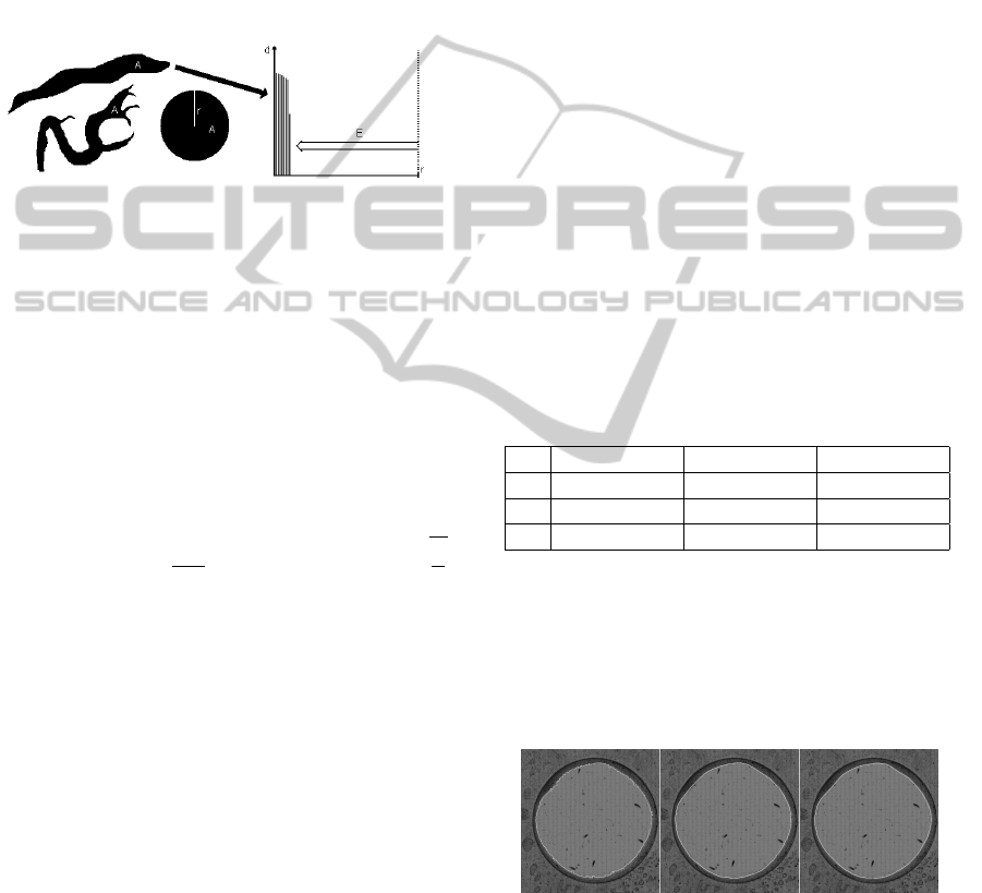
5.
Figure 5: From left to right: Thin objects and a circle with
identical areas followed by the corresponding normalized
histogram relative to the circle radius with the empty bin
amount E are illustrated.
At first, a distance transform is applied on C
t
and
the area A is calculated. All distances are normalized
relative to the radius r of the circle. A second nor-
malization is done, so that r = 255. The distances
are represented in a histogram with 256 bins. Begin-
ning at the maximal histogram value (255), the empty
bins E are counted in direction of the histogram ori-
gin. Finally, a threshold T
f
is used for the detection
as follows:
Ω
t
= {C|∀C ∈ Ω
ZC
:
E
255
> T
f
}; relative to r =
r
A
π
(3)
A good threshold for the detection is T
f
= 0.6.
4.5 Zooplankton Recognition
The recognition is not the major part of our contri-
bution. Nevertheless, we explain it in short to com-
plete the argumentation. In our scenario, the set Ω
ZC
0
is used for zooplankton species recognition. For ev-
ery segment 52 features are extracted. The best fea-
tures are selected by an automatic selection approach.
Classification is done with an SVM. The classifica-
tion result is improved manually by an zooplankton
expert with few user interactions. The improved result
is stored and used for training an improved classifier.
5 RESULTS
We evaluated the steps chamber segmentation (B),
candidate segmentation (C) and pre-classification (D)
separately. The steps (C) and (D) are performed on
the results produced with the best method of step (B).
All results are compared with ground truth data gener-
ated by a zooplankton expert, who analyzed the sam-
ple, marked all existing specimen with a bounding
box and classified them. For our evaluation five large
images with ground truth data were available with fol-
lowing properties:
1. image 1: 62520×62000 pixels, 30×40 tiles
2. images 2,3,4: 64604×66650 pixels, 31×43 tiles
3. image 5: 89612×89900 pixels, 43×58 tiles
5.1 Chamber Segmentation
To evaluate the chamber segmentation, we segmented
the chamber in all images manually and compared it
to the automatic chamber segmentation results. For
the three chamber segmentation methods, we calcu-
late precision, recall and f-score. A value of 1 indi-
cates a perfect segmentation. The standard deviations
according to the evaluation measures are illustrated in
brackets. The evaluation of the three chamber seg-
mentation methods is presented in table 2.
Table 2: Chamber segmentation evaluation of the longest
contour (lc), active contours (ac) and region growing (rg)
approach.
precision recall f-score
lc 0.889 (13.5) 0.991 (0.36) 0.927 (8.66)
ac 0.993 (0.14) 0.997 (0.11) 0.995 (0.09)
rg 0.996 (0.17) 0.995 (0.67) 0.996 (0.27)
As can be seen in table 2, the active contour
and region growing approach lead to the best re-
sults. However, region growing is slightly better. The
longest contour approach leads to the worst results
with an extracted contour that can be a little bit frayed.
Images of the results can be seen in figure 6.
Figure 6: The images show the results of our three ap-
proaches for chamber contour detection. From left to right:
The longest contour, the active contour and the region grow-
ing approach are pictured.
VISAPP2014-InternationalConferenceonComputerVisionTheoryandApplications
422
5.2 Zooplankton Segmentation
The segments of the set Ω
ZC
are compared to the
ground truth (manually marked bounding boxes). In
Ω
ZC
are zooplankton and non-zooplankton segments.
We only calculate the number of missing zooplankton
segments in Ω
ZC
, because the separation in zooplank-
ton and non-zooplankton segments is done in a later
step. In summary, only 0.5% of the ground truth were
missing after segmentation.
5.3 Zooplankton Pre-Classification
We evaluate the pre-classification algorithm by com-
paring the final set Ω
ZC
0
with the ground truth zoo-
plankton data. For the sets Ω
t
and Ω
qr
an evaluation is
only possible by subjective manual estimation. Evalu-
ated by our visual judgment, the sets contain correctly
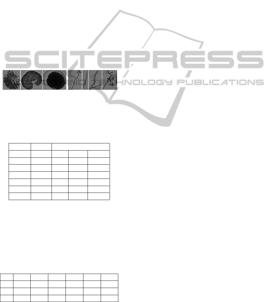
classified thin and quasi round objects (see figure 7).
Figure 7: The left images picture quasi round and the right
thin objects. The contour of the segment is drawn in white.
The amount of classified segments per image is
shown in table 3.
Table 3: Number of segments pre-classified as thin (Ω
t
),
quasi-round (Ω
qr
) and zooplankton candidate (Ω
ZC
0
).
image input output
I
in
|Ω
ZC
| |Ω
t
| |Ω
qr
| |Ω
ZC
0
|
1 342 61 27 254
2 361 103 30 228
3 416 71 37 308
4 337 45 39 253
5 644 156 67 421
sum 2100 436 200 1464
The final set Ω
ZC
0
contains zooplankton and non-
zooplankton segments. We evaluate the binary classi-
fication case with the measures specificity, precision
and recall (see table 4), whereby the best possible
value is 1. As can be seen, the specificity and pre-
cision of our pre-classification approach is very good,
Table 4: Specificity (sp), precision (pr) and recall (re) of the
reduced zooplankton candidate set Ω
ZC
0
1 2 3 4 5 All
sp 0.94 0.97 0.97 0.95 0.95 0.96
pr 0.96 0.96 0.98 0.97 0.94 0.96
re 0.48 0.43 0.40 0.49 0.43 0.44
but the recall is not. In other words, the set Ω
ZC
0
con-
tains nearly all zooplankton segments, but contains
some non-zooplankton segments, too.
6 CONCLUSION AND FUTURE
WORKS
We presented a novel approach to segment and pre-
classify zooplankton located in a counting chamber
in very large images. It is the first approach in the
field of zooplankton recognition that is able to deal
with images larger than the available main mem-
ory of standard computers. We outlined how three
different methods can be used to detect the count-
ing chamber and one method to segment the zoo-
plankton with a contour based Split & Merge ap-
proach. The segmentation result contains zooplank-
ton and non-zooplankton segments. To reduce the
non-zooplankton species, we presented a solution for
pre-classifying the segments. The classification algo-
rithm can detect thin and quasi round objects. For
the thin object detection, a novel approach was intro-
duced allowing a detection independently of the ob-
ject shape and rotation. The chamber detection eval-
uation shows very good results. The evaluation of
the zooplankton segmentation and pre-classification
show that there are non-zooplankton segments that re-
main undetected.
Our current work focuses on detecting these non-
zooplankton segments by using the segmentation and
pre-classification results. We are training one or
more classes representing non-zooplankton and we
are working on a multi resolution segmentation by
using the implemented quadtree. For the recognition
we plan to adapt and to develop special shape fea-
tures like in (Seng, 2013). To extend the system and
to be able to segment every zooplankton species with-
out exception an user-driven semi-automatic segmen-
tation like active contours in (Kass et al., 1988) and
(Ahmed et al., 2013) is planned.
ACKNOWLEDGEMENTS
We thank Joerg Voskamp, Arjan Kuijper, An-
dreas Fricke and Martin Feike. This paper con-
tains results of the research project ZooCount (no.
KF2212904KM0). ZooCount was funded by the Cen-
tral Innovation Program for SMEs, Federal Ministry
of Economics and Technology, Germany.
ContourbasedSplitandMergeSegmentationandPre-classificationofZooplanktoninVeryLargeImages
423

REFERENCES
Ahmed, F., Le, H., Olivier, J., and Bon, R. (2013). An ac-
tive contour model with improved shape priors using
fourier descriptors. VISAPP 2013 - Proceedings of the
International Conference on Computer Vision Theory
and Applications, 1:472–476.
Chehdi, K., Boucher, J., and Hillion, A. (1986). Automatic
classification of zooplancton by image analysis. In
Acoustics, Speech, and Signal Processing, IEEE In-
ternational Conference on ICASSP ’86., volume 11,
pages 1477 – 1480.
Culverhouse, P., Williams, R., Simpson, B., Gallienne, C.,
Reguera, B., Cabrini, M., Fonda-Umani, S., Parisini,
T., Pellegrino, F., Pazos, Y., Wang, H., Escalera,
L., Moroo, A., Hensey, M., Silke, J., Pellegrini, A.,
Thomas, D., James, D., Longa, M., Kennedy, S., and
del Punta, G. (2006). Hab buoy: a new instrument for
in situ monitoring and early warning of harmful al-
gal bloom events. African Journal of Marine Science,
28(2):245–250.
Davis, C. S., Gallager, S. M., Bermann, N. S., Haury,
L. R., and Strickler, J. R. (1992). The video plank-
ton recorder (vpr): design and initial results. In Arch.
Hydrobiol. Beith., volume 36, pages 67–81.
Davis, C. S., Thwaites, F. T., Gallager, S. M., and Hu, Q.
(2005). A three-axis fast-tow digital video plankton
recorder for rapid surveys of plankton taxa and hy-
drography. Limnology and Oceanography-Methods,
3:59–74.
Dubelaar, G. and Jonker, R. (2000). Cytobuoy: a step
forward towards using flow cytometry in operational
oceanography. Sci. Mar., 64(2):255–265.
Fawell, J. (1976). Electronic measuring devices in the sort-
ing of marine zooplankton. In zooplankton fixation
and preservation, pages 201 – 206. Ed. by H.F. Steed-
man, Paris:UNESCO Press.
Gaston, K. J. and O’Neill, M. A. (2004). Automated species
identification: why not? Philosophical Transactions
of the Royal Society of London Series B-Biological
Sciences, 359(1444):655–667+.
Gorsky, G. and Grosjean, P. (2003). Qualitative and quanti-
tative assessment of zooplankton samples. GLOBEC
INTERNATIONAL NEWSLETTER APRIL, 9.
Herman, A. W. and Dauphinee, T. M. (1980). Continu-
ous and rapid profiling of zooplankton with an elec-
tronic counter mounted on a batfish vehicle. Deep
Sea Research Part A. Oceanographic Research Pa-
pers, 27(1):79 – 96.
Jeffries, H., Berman, M., Poularikas, A., Katsinis, C.,
Melas, I., Sherman, K., and Bivins, L. (1984). Auto-
mated sizing, counting and identification of zooplank-
ton by pattern recognition. Marine Biology, 78:329–
334.
Kass, M., Witkin, A., and Terzopoulos, D. (1988). Snakes:
Active contour models. INTERNATIONAL JOURNAL
OF COMPUTER VISION, 1(4):321–331.
Katsinis, C. (1979). Digital Image Processing and Identifi-
cation of Zooplankton. University of Rhode Island.
Kelkar, D. and Gupta, S. (2008). Improved quadtree method
for split merge image segmentation. In Emerging
Trends in Engineering and Technology, 2008. ICETET
’08. First International Conference on, pages 44 –47.
Luo, T., Kramer, K., Samson, S., Remsen, A., Goldgof,
D. B., Hall, L. O., and Hopkins, T., editors (2004).
Active learning to recognize multiple types of plank-
ton, volume 6. IEEE.
Olson, R. J. and Sosik, H. M. (2007). A submersible
imaging-in-flow instrument to analyze nano- and mi-
croplankton: Imaging FlowCytobot. Limnology and
Oceanography: Methods, 5:195–203.
Otsu, N. (1979). A Threshold Selection Method from Gray-
level Histograms. IEEE Transactions on Systems,
Man and Cybernetics, 9(1):62–66.
Picheral, M., Guidi, L., Stemmann, L., Karl, D., Iddaoud,
G., and Gorsky, G. (2010). The underwater vision pro-
filer 5: An advanced instrument for high spatial reso-
lution studies of particle size spectra and zooplankton.
Limnology and Oceanography: Methods, 8:462–473.
Samson, S., Hopkins, T., Remsen, A., Langebrake, L., Sut-
ton, T., and Patten, J. (2001). A system for high-
resolution zooplankton imaging. Oceanic Engineer-
ing, IEEE Journal of, 26(4):671 –676.
Seng, L. (2013). Contour-based shape recognition using
perceptual turning points. VISAPP 2013 - Proceed-
ings of the International Conference on Computer Vi-
sion Theory and Applications, 1:487–491.
Sheldon, R. and Parsons, T. R. (1967). A practical manual
on the use of the Coulter counter in marine research.
Coulter Electronics Sales.
Sieracki, C. K., Sieracki, M. E., and Yentsch, C. S. (1998).
An imaging-in-flow system for automated analysis of
marine microplankton. Marine Ecology Progress Se-
ries, 168:285–296.
Toth, L. and Culverhouse, P. F. (1999). 3d object recogni-
tion from static 2d views using multiple coarse data
channels. Image Vision Comput., 17(11):845–858.
Tsechpenakis, G., Guigand, C. M., and Cowen, R. K., edi-
tors (2007). Image Analysis Techniques to Accompany
a new In Situ Ichthyoplankton Imaging System. IEEE.
Tsechpenakis, G., Guigand, C. M., and Cowen, R. K.
(2008). Machine vision-assisted in-situ ichthyoplank-
ton imaging system. Sea Technology, 49(12):15–20.
Website (2013a). http://www.fluidimaging.com.
Website (2013b). http://www.hydroptic.com/uvp.html.
Website (2013c). http://www.zooscan.com.
VISAPP2014-InternationalConferenceonComputerVisionTheoryandApplications
424
