FREQUENCY SPECTRUM OF THE WAVE BACKSCATTERED
TO TRANSCEIVER MOVING TOWARDS ROUGH SURFACE
Alexander B. Shmelev
Radiotechnical Institute by Academician A.L.Mints, 8 Marta Str.,Bld.10-1, Moscow, 127083, Russia
Keywords: Frequency spectrum, randomly rough surface, aerospace vehicle, incident wave, scattered field,
characteristic function, correlation function, normal distribution.
Abstract: Frequency spectrum of the wave scattered by randomly rough surface back to transceiver located on
aerospace vehicle moving towards the surface is evaluated and investigated in explicit form. Kirchhoff’s
(physical optics) method is applied for scattered field evaluation. It is assumed that transceiver irradiates
directive spherical wave illuminating circled area on the surface. Distribution of the rough surface height is
assumed to be normal with isotropic Gaussian correlation function. Application the effective approximation
formula for characteristic functions difference in integrand gives rise to spectrum evaluation for arbitrary
height of surface irregularities. Frequency spectrum is shown to exist in two forms. The first one is
represented by monotonic curve, depending on correlation distance of the rough surface. The second form
includes one maximum, which position and amplitude are related with the roughness’ mean square slope.
On the parameter plane the curve is plotted which separates regions with abovementioned spectrum forms.
1 INTRODUCTION
The purpose of this paper is theoretical evaluation
frequency spectrum of radiowave backscattered to
transceiver moving towards randomly rough surface.
This situation occurs, for example, before spacecraft
landing on the Moon or planet surface. Irregularities
of such surfaces are formed by natural factors and
may be described as random fields. Frequency
spectrum provides information about statistical
characteristics of rough surface, such as correlation
distance, mean square height and slope of its
irregularities.
The scattering problem on randomly rough
surface may be formulated as follows. Let scalar
(sound) or vector (electromagnetic) wave fall on the
surface S separating two media. The surface is
described by equation
(, ,)zxyt=
ζ
, where ζ is
random function of coordinates x, y and time t. It is
required to establish relation between statistical
parameters of rough surface and characteristics of
scattered field. Approaches to this problem as well
as results obtained were described in literature at
various times (Beckman and Spizzichino, 1963),
(Bass and Fuks, 1972), (Shmelev, 1972).
Nevertheless this problem is actual up to now
because of application peculiarity variety.
We use in this paper Kirchhoff’s (physical
optics) method – the most developed and effective in
wave scattering problems. It is based on assumption
that reflection of incident wave at every point of
rough surface locally obeys geometric optics laws.
This means that our consideration is restricted to
rather smooth and gentle irregularities, which
curvature radius is large in comparison with wave
length. We don’t take into account shadowing
effects, so surface slopes are assumed to be not too
sharp.
The problem solution by Kirchhoff’s method is
used to include two stages. At the first stage
dynamical part of the problem is considered.
General expression for wave field diffracted on the
surface S is composed in Kirchhoff’s approximation.
The surface height is described herein by arbitrary
function
(, ,)
z
xyt
=ζ
. At the second stage this
function is declared to be random and various
statistical characteristics of scattered field, such as
middle value, average intensity, correlation function
etc., are evaluated by averaging over rough surfaces
ensemble. In this paper we are interested in
frequency spectrum of backscattered field when
transceiver is moving towards rough surface (in
15
B. Shmelev A.
FREQUENCY SPECTRUM OF THE WAVE BACKSCATTERED TO TRANSCEIVER MOVING TOWARDS ROUGH SURFACE.
DOI: 10.5220/0004784600150020
In Proceedings of the Second International Conference on Telecommunications and Remote Sensing (ICTRS 2013), pages 15-20
ISBN: 978-989-8565-57-0
Copyright
c
 2013 by SCITEPRESS – Science and Technology Publications, Lda. All rights reserved

vertical direction). Analogous problem in the case
when transceiver is moving along rough surface (in
horizontal direction) was studied earlier (Shmelev,
1973). More accurate explicit results may be
obtained in the case under consideration.
2 DYNAMICAL PART
For the sake of simplicity we consider scalar (sound)
waves taking in mind that vector character of
electromagnetic wave acts on polarization but not on
spectrum shape. Let the directional spherical wave
0
0
()
() e
ik
r
F
−
Φ=
−
rR
n
r
rR
(1)
fall on the rough surface S which height
(, )zxy
=ζ
diverges from the mean plane
(
)
,0zxy=ζ =
denoted by S
0
. The wave number in upper medium is
kc=ω , directivity pattern of transmitter is ()
r
F n ,
where
0
0
r
−
=
−
rR
n
rR
,
0
R - transmitter position vector.
At first we consider motionless surface S. Its
movement towards transceiver will be taken into
account in quasi-static approximation by time
dependence restoration in final expression for
diffracted field. This approximation is valid if
transmitter velocity is small in comparison with light
velocity
vc
. Geometric scheme of the wave
scattering problem is shown on Figure 1 for general
case of spaced transmitter Q and receiver P.
Figure 1: The scattering problem geometry for spaced
transmitter and receiver.
Here R
0
and R are transmitter Q and receiver P
position vectors,
(, ,(, )) ( ,)xy xy
⊥
=
ζ
=
ζ
rr is radius
-vector of rough surface point, n - surface normal at
this point.
Diffracted field at observation point P is related
with values of the field φ and its normal derivative
n
∂
ϕ∂ on the rough surface S by Green’s formula
1e e
()
4
ik ik
S
dS
nn
−−
⎛⎞
∂∂ϕ
ϕ= ϕ −
⎜⎟
⎜⎟
π∂−∂−
⎝⎠
∫
Rr Rr
R
Rr Rr
. (2)
In Kirchhoff’s approximation following relations
are valid at the every point of surface S
,VV
nn
∂
ϕ∂Φ
ϕ= Φ =−
∂
∂
, (3)
where
(, )VV
=
rn is local Fresnel reflection
coefficient. Substitution (1) and (3) into (2) gives
()
0
0
e
1
()
4
ik ik
r
S
F
VdS
n
+−
⎡
⎤
∂
ϕ=
⎢
⎥
π∂ −⋅−
⎢
⎥
⎣
⎦
∫
r-R R r
n
R
RrrR
. (4)
Let us assume now that transmitter and receiver
are situated far enough from the rough surface, so
that
2
0
,,,RR k
λ
σσ
, where σ is mean square
height of surface irregularities and
2 kλ= π - wave
length. Then we separate two types of multipliers in
(4) – rapidly oscillating exponent and slowly varying
functions weakly dependent on rough surface height
(
)
⊥
ζ r
. Setting
0
ζ
=
in this functions, keeping
linear with respect to
ζ
terms in exponent power
expansion and changing integration over surface S
by integration over middle plane S
0
, we come to
known expression for diffracted field
()
01 1
0
2
2
01
01 1
e
() e
4
z
ikR ikR
iq
z
S
iq
VF d
RR q
+
ζ
⊥
ϕ=
π
∫
Rn r
, (5)
where
(
)
01 0 1
,,0, , ,xy
⊥⊥⊥
==−=−rRrRRRr
01 01 01 1 1 1
,RR
=
=nR nR and
()
01 1
k=−qnn
is
the scattering vector.
Let us now take into consideration motion of the
rough surface along z-axis with the constant velocity
v. In quasi-static approximation we have to set in (5)
(
)
(
)
,tvt
⊥⊥
ζ
=
ζ
=
ζ
+rr. In addition we assume that
surface S is absolutely reflecting (V=1) – absolutely
rigid in acoustics or perfectly conductive in
electrodynamics. This removes influence of surface
Second International Conference on Telecommunications and Remote Sensing
16

material properties on spectrum under investigation.
Solution of dynamical part of the problem takes on
final form
()
()
()
01 1
0
0
2
2
01
01 1
ee
e
4
zz
ik R R
it
iq iq vt
z
S
iq
F
d
RR q
⊥
+
ω
ζ+
⊥
ϕ=
π
∫
r
nr
. (6)
This expression provides basis for further evaluation
statistical characteristics of diffracted field.
3 AVERAGE FIELD
Averaging expression (6) over ensemble of random
field
()
⊥
ζ r
realizations leads to average value of
diffracted field
()
()
01 1
0
0
2
2
1
01 1
ee
e
4
z
ik R R
it
iq vt
z
z
S
iq
Ffqd
RR q
+
ω
ζ
⊥
ϕ=
π
∫
r
, (7)
where corner brackets denote averaging operation,
(
)
(
)
1
exp
zz
fq iq
ζ
=ζ
is characteristic function of
the rough surface S. We suppose that random field
()
⊥
ζ r
is statistically homogeneous.
Evaluation this integral by means of stationary
phase technique gives physically transparent result
()
(0)
1
(,) ( ) ()exp
zs zs
tfq iqvt
ζ
ϕ= ϕRR
, (8)
where
2cos
z
ss
qk=θ is z-component of scattering
vector at stationary point coinciding with the point
of mirror reflection from the mean plane S
0
. This
point is chosen to be origin of coordinates. Incidence
angle at stationary point is denoted by
s
θ . The field
mirrored from the plane S
0
is designated as
(
)
(
)
0
ϕ R .
Average field is interpreted like coherent part of
diffracted field. Multiplier
()
1
z
s
f
q
ζ
is effective
reflection coefficient of average field. If surface
height is distributed under Gaussian law, it has the
form
(
)
2
22 2 2
1
( ) exp 2 cos e
zs s
fq k
−Δ
ζ
=−σ θ=
,……(9)
where
2cos
s
kΔ= σ θ is the Rayleigh parameter
characterizing degree of surface roughness.
Doppler shift of average field is equal to
2cos
z
ss
qv kv
Δ
ω= = θ . (10)
Backscattering case follows by setting
0
s
θ= in
formulas obtained.
4 SCATTERED FIELD
Scattered field is meant to be diffracted field minus
its average value
Δϕ
=
ϕ
−
ϕ
. Let us evaluate
temporal correlation function of the scattered field
(
)
(
)
(
)
,,tt t t
∗
′
′
ψ− =Δϕ ⋅Δϕ
RR
. Using (6) and (7)
we obtain
()
()
()
0
0
2
4
01
2
2222
01 1
e
e
16
z
i
iq v
z
S
Fq
Jd
RRq
ωτ
τ
⊥
ψτ=
π
∫
n
qr
, (11)
where
() ( ) ( )
2
2
21
,, e
i
zz z
J
fqq fq d
⊥
∞
ζζ
−∞
⎡⎤
=−−
⎢⎥
⎣⎦
∫
q ρ
q ρρ
,(12)
(
)
(
)
(
)
2
,, expfuw iu iw
ζ⊥⊥
=ζ+ζ+
⎡
⎤
⎣
⎦
ρ rrρ
is two-
dimensional characteristic function of the rough
surface.
Integral
(
)
J
q
is well studied in cited literature.
There are known its explicit expressions for
irregularities distributed under Gaussian law. In the
case of small irregularities in comparison with the
wave length
()
2
1kδ= σ 
and Gaussian spatial
correlation coefficient
(
)
()
22
expKlρ= −ρ
with the
single correlation distance l this expression has the
form
(
)
(
)
22 2 22
exp 4 , 1
z
Jlqql
⊥
=πσ − δq 
. (13)
In the opposite case of high irregularities
1δ  and
arbitrary spatial single-scale correlation function
integral J equals to
()
2
22
4
exp , 1
zz
q
J
qq
⊥
⎛⎞
π
=−δ
⎜⎟
ββ
⎝⎠
q 
, (14)
where parameter
(
)
22 22
204
s
K
l
′′
β=σ =− σ = σ
characterizes mean-square slope of the surface
roughness.
Frequency Spectrum of the Wave Backscattered to Transceiver Moving Towards Rough Surface
17

In this paper we use the integral J evaluation
technique valid for arbitrary values of parameter δ,
i.e. for arbitrary height of surface irregularities. It is
based on approximation formula
()
()
2
2
exp 1 e e 1 e exp
1e
x
x
−−γ −γ
−γ
⎛⎞
γ
⎡⎤
−γ − − − −
⎜⎟
⎣⎦
−
⎝⎠

, (15)
where γ is positive parameter. This approximation
was studied in detail in (Vinogradov and Shmelev,
2008).
Let us assume that the surface height is
distributed under Gaussian law with Gaussian spatial
correlation coefficient
(
)
(
)
22 2 2
exp
x
xyy
Kll=−ρ−ρρ
taking into consideration possible non-isotropy of
surface irregularities. Difference of characteristic
functions in integrand (12) may be represented in
accordance with (15) by following expression
()()
(
)
()
()
()
22 22
22
2
21
22 22
22 22
,,
exp 1 e exp
1e exp ,
xx yy
z
zz z
ll
zz
q
xx yy
fqq fq
qq
ll
ζζ
−ρ −ρ
−σ
ΦΦ
−− =
⎡⎤
=−σ− −−σ
⎢⎥
⎣⎦
−−ρ−ρ
ρ


(16)
where effective correlation distances have the values
() ()
22 22
2
2
22
22 22
1e , 1e
zz
y
qq
x
xy
zz
l
l
ll
qq
−σ −σ
ΦΦ
=− =−
σσ
, (17)
dependent on wave length.
Substitution (16)-(17) into (12) and immediate
evaluation of the integral lead to result
()
()
22
22 22
1e exp .
4
z
xx yy
q
xy
ql ql
Jll
ΦΦ
−σ
ΦΦ
⎛⎞
+
π− −
⎜⎟
⎜⎟
⎝⎠
q 
(18)
In the case of statistically isotropic surface we
have to set
xy
lll==
. This gives
()
()
()
22
22
22
2
2
2
22
1e exp ,
4
1e .
z
z
q
q
z
ql
Jl
l
l
q
−σ
⊥Φ
Φ
−σ
Φ
⎛⎞
=π − −
⎜⎟
⎝⎠
=−
σ
q
(19)
In limiting cases of small and high irregularities
these expressions lead to (13) and (14).
Let us consider now backscattering case, when
transmitter and receiver positions coincide, i.e.
(
)
0
0, 0,
Z
==RR
. Let rough surface be statistically
isotropic, and multiplier describing antenna pattern
be in the form
()
2
01
1, if ,
0, if ,
ra
F
ra
⊥
⊥
≤
⎧
=
⎨
>
⎩
n
(20)
where a is radius of illuminated area on the mean
plane S
0
. Transformation to polar coordinates in
integrand (11) gives then required expression for
temporal correlation function of backscattered field
() ()
0
2
4
2222
01 1
00
e
e
16
z
a
i
iq v
z
q
drdr J
RRq
π
ωτ
τ
⊥⊥
ψτ= ϕ
π
∫∫
q
, (21)
where following relations are valid:
(
)
()
()
2222
01 1 1 01
22
01
22
22 2
22 2
2
22 2 2 2
,, ,
,
22 , 4,
4
1exp .
4
Z
RRrZ
Z
kk qk
rZ
lr Z
kZ
l
kZ rZ
⊥⊥
⊥
⊥
⊥
Φ
⊥
=− = − = = +
−
== =
+
+
⎡
⎤
⎛⎞
σ
=−−
⎢
⎥
⎜⎟
σ+
⎢
⎥
⎝⎠
⎣
⎦
RRr
r
qn
(22)
5 FREQUENCY SPECTRUM
As is known, frequency spectrum may be evaluated
by Fourier transformation of temporal correlation
function
() ()
e
i
Gd
∞
ωτ
−∞
ω
=ψτ τ
∫
. (23)
Insertion (21), (22) into (23) and application of δ-
function integral representation
()
1
e
2
i
d
∞
ωτ
−∞
δω= τ
π
∫
gives following expression for frequency spectrum
of backscattered field
()
(
)
()
4
0
222
01 1
0
1
4
a
z
z
qJ
Gqvrdr
RRq
⊥⊥
ω= δω−ω−
∫
q
. (24)
Introducing new integration variable
22
2
z
kvZ
xqv
Z
r
⊥
==−
+
and performing integration of
Second International Conference on Telecommunications and Remote Sensing
18

δ-function, we obtain frequency spectrum of
backscattered field in explicit form
()
(
)
()
()
2
2
2
2
23 2
1e
1
exp 1 e
2
G
kvZ
−δΩ
−δΩ
π−
⎡
⎤
Ω−
⎢
⎥
Ω= −
βΩ βΩ
⎢
⎥
⎣
⎦
. (25)
Dimensionless frequency
0
22kv kv
ω−ω
Δω
Ω= =
varies
within
cos 1θ≤Ω≤ , where angle 2θ is the beam
width of transmitter, so that
tan aZθ= . Beyond
this interval
()
0.G Ω≡
Physically this means that
frequency spectrum includes all possible Doppler
shifts of scattered field – from maximum
max
2kvΔω = in vertical direction till minimum
min
2coskvΔω = θ in direction of illuminated area
border.
To avoid dependence on inessential parameters
let us consider spectrum normalized to its value at
Ω=1, i.e.
() () ()
0
1GGGΩ= Ω
:
()
()
()
()
()
2
2
2
2
0
22
3
1e
1
exp 1 e
1e
G
−δΩ
−δΩ
−δ
−
⎡
⎤
Ω−
⎢
⎥
Ω= −
βΩ
⎢
⎥
−Ω
⎣
⎦
.(26)
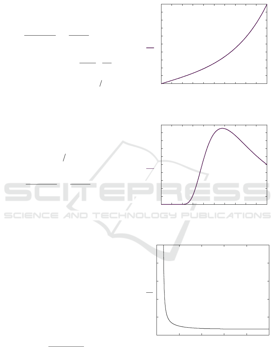
Analysis of this expression shows that there exist
two forms of frequency spectrum. The first one is
represented by monotonic curve, depending on
correlation distance of the rough surface. The second
form includes one maximum, which position and
amplitude are related with irregularities mean square
slope. Typical examples of these spectrum forms are
shown on Figures 2 and 3.
Regions on the plane (δ,β) corresponding to one
or another form of spectrum differ in sign of
derivative
()
0
1G
′
. Region, where
(
)
0
10G
′
>
,
corresponds to the first form and region, where
()
0
10G
′
< , – to the second form. The curve
corresponding to
()
0
10G
′
=
separates these two
regions. Simple calculations using (26) lead to
equation of this curve plotted on Figure 4:
()
()
2
21 e
334e
−δ
−δ
−
β=
−+δ
. (27)
0 0.1 0.2 0.3 0.4 0.5 0.6 0.7 0.8 0.9 1
0
0.1
0.2
0.3
0.4
0.5
0.6
0.7
0.8
0.9
1
G
0
u()
u
Figure 2: The first form of frequency spectrum for
parameter values δ=0.1, β=0.1.
0 0.1 0.2 0.3 0.4 0.5 0.6 0.7 0.8 0.9 1
0
0.2
0.4
0.6
0.8
1
1.2
1.4
1.6
1.8
2
G
0
u()
u
Figure 3: The second form of frequency spectrum for
parameter values δ=100, β=2.
0 2 4 6 8 10
0
2
4
6
8
10
βδ()
δ
Figure 4: The curve separating regions with the first
(under the curve) and the second (above the curve) forms
of spectrum.
Frequency Spectrum of the Wave Backscattered to Transceiver Moving Towards Rough Surface
19

The first spectrum form results in the case when
irregularities are rather small
()
1δ<
or gentle
()
0.7β< . High and sharp irregularities lead to the
second form of spectrum.
In the case of extreme low roughness
(
)
1δ 
expression (26) is simplified to
()
(
)
2
0
exp 1 , 1G
⎡⎤
ΩΩ⋅ −α−Ω δ
⎣⎦
, (28)
where
()
2
klα=δβ=
is mean square correlation
distance in the scale of wave length. Differentiation
(28) gives relation
()
0
11
2
G
′
−
α=
, (29)
which may be used for experimental estimation of
parameter α.
In the opposite case of very high roughness
()
1δ 
expression (26) takes on the form
()
(
)
2
0
32
1
1
exp , 1.G
⎡⎤
−Ω
⎢⎥
Ω= − δ
ΩβΩ
⎢⎥
⎣⎦
 (30)
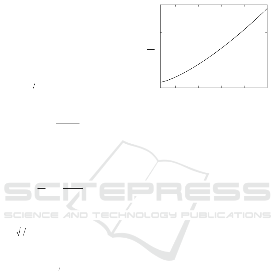
For sharp irregularities
()
0.67β> it describes
the second spectrum form having maximum at
()
23
m
Ω= β
. Thus position of maximum carries
information on mean square slope of the rough
surface β. Additional information on this parameter
contains height of this maximum
()
32
0
332
exp
22
m
G
⎛⎞
ββ−
⎛⎞
Ω= ⋅ −
⎜⎟
⎜⎟
β
⎝⎠
⎝⎠
. (31)
This function is plotted on Figure 5.
2 4 6 8 10
0
5
10
15
G
0
β()
β
Figure 5: View of the function (31).
6 CONCLUSIONS
Proposed evaluation the frequency spectrum of the wave
backscattered from rough surface in explicit form and for
arbitrary roughness height lets us establish detailed
relations between spectrum parameters and statistical
characteristics of the surface. Results obtained may be
useful for further development of rough surfaces remote
sensing technique.
REFERENCES
Beckman, P. and Spizzichino, A., 1963. The Scattering of
Electromagnetic Waves from Rough Surfaces.
Pergamon Press. New York.
Bass, F.G. and Fuks, I.M., 1972. Wave Scattering on
Statistically Rough Surface. Nauka Press. Moscow. (In
Russian).
Shmelev, A.B., 1972. Wave Scattering by Statistically
Uneven Surfaces. American Institute of Physics
Incorporated: Soviet Physics Uspekhi, 15, 173-183.
Shmelev, A.B., 1973. The Frequency Spectrum of a Sound
Field Scattered by a Uniformly Moving Rough
Surface. Izvestiya VUZov (Radiofizika), 16, 54-61.
(In Russian).
Vinogradov, A.G. and Shmelev, A.B., 2008. Wave
Scattering by a Rough Surface in Random
Inhomogeneous Medium. Radiotechnika Press:
Electromagnetic Waves and Electronic Systems,
13(9), 38-45. (In Russian).
Second International Conference on Telecommunications and Remote Sensing
20