
Computational Fluid Dynamic Solver based on Cellular
Discrete-Event Simulation
Michael Van Schyndel, Gabriel Wainer and Mohammad Moallemi
Dept. of Systems & Computer Engineering, Carleton University, Ottawa, ON, Canada
Keywords: Cell-DEVS, Computational Fluid Dynamics.
Abstract: Computational Fluid Dynamics (CFD) deals with computing the equations of fluid flows using numerical
methods. The Discrete-Event System specification (DEVS) theory has been used to approximate the contin-
uous systems by applying a quantized state system approach. In this research, we employ Cellular DEVS
theory (Cell-DEVS) – originally proposed for modeling and simulation of spatial environments – to create a
uniform set of rules for CFD. This harmonized set of state changes can effectively render the fluid dynam-
ics, by applying the accurate rule that represents the behavior of the fluid. The combination of the simplicity
and the mathematical backbone allows for constructing models computable on an average computer or an
array of cluster computers.
1 INTRODUCTION
Computational Fluid Dynamics (CFD) solving is re-
ferred to the research on numerical methods and al-
gorithms to solve and analyze the movement and in-
teractions of fluid flows (Anderson, 2009).. In gen-
eral, no analytical solution exists for non-linear fluid
models; hence, the numerical approximation methods
also called “computational models” come to play.
CFD Solvers are required to process a large number
of computations, which makes the use of computer-
based approaches inevitable. In a computerized pro-
cessing of CFD, a boundary for the problem is de-
fined and the environment is divided into cellular
spaces, each of them representing a physical volume.
The laws of motion are defined based on equations of
motion, enthalpy, radiation, and species conserva-
tion. The behavior of the fluid at the boundaries is al-
so defined, which is called boundary conditions.
These specifications construct a model of the fluid,
which can be simulated on a computing device. Fi-
nally, visualization and analysis of the results can
render a meaningful and sensible outcome of the
computations. Different cellular methods have been
proposed to solve these problems. In particular, Cel-
lular automata (CA) theory (Ilachinski, 2001) is a
branch of discrete dynamic systems, in which space
is represented by a cellular grid, with each cell being
a state machine. In CA the time advances in a dis-
crete manner, triggering state changes in the cells,
based on the value of their neighbor cells. CA have
been used in physics, complexity science, theoretical
biology, microstructure modeling, etc.
The Cell-DEVS formalism (Wainer, 2009) is an
improved derivative of CA, which solves the prob-
lem of unnecessary processing burden in cells and al-
lows efficient asynchronous execution, using a con-
tinuous time-base, and without losing accuracy. In
this methodology, each cell is represented as DEVS
atomic models (Zeigler and Praeofer Kim, 2000) that
changes states in an event-driven fashion. In this re-
search, we propose using Cell-DEVS to implement
CFD equations to simulate fluid dynamics. The rule-
based nature of cellular model behavior definition
provides a platform for area-wise behavior definition,
leading to easier and faster experimentation of CFD
solvers. The other advantage of this method is its fast
computing apparatus working asynchronously on the
cellular grid, increasing the execution speed. The
continuous time-advance nature of Cell-DEVS can
contribute to the seamless simulation of CFD, in
comparison with the discrete timing in CA that lacks
the smoothness of fluid flow. The model can be able
to provide realistic results with reasonable speed. Fi-
nally, the formal I/O port definitions in the formalism
permits producing output signals based on specific
condition satisfaction in the cell lattice, allowing for
data transfer between different spatial components.
The CD++ tool (Wainer, 2009) provides a devel-
opment environment to create and navigate through
217
Van Schyndel M., Wainer G. and Moallemi M..
Computational Fluid Dynamic Solver based on Cellular Discrete-Event Simulation.
DOI: 10.5220/0004593902170223
In Proceedings of the 3rd International Conference on Simulation and Modeling Methodologies, Technologies and Applications (SIMULTECH-2013),
pages 217-223
ISBN: 978-989-8565-69-3
Copyright
c
2013 SCITEPRESS (Science and Technology Publications, Lda.)

the process of Modeling and Simulation (M&S) of a
Cell-DEVS model. CD++ is an open-source frame-
work that has been used to model environmental,
biological, physical and chemical models as well as
many other real-life simulations. The toolkit includes
a high-level scripting language keyed to Cell-DEVS,
a simulation engine, a testing interface and 2D and
3D graphical interfaces.
The solver proposed here provided results that are
realistic and achieve the goals stated. We will discuss
how the framework can be used and how to export
the generated data to graphical environments.
2 RELATED WORK
Fluid dynamic solvers are used for a wide variety of
purposes. Their goal is to create a realistic represen-
tation of a naturally occurring fluid system such as
smoke rising or dust blowing. The flow of fluids can
be viewed as solid particles interacting with velocity
fields or as densities. There are different methods to
solve some CFD; Lattice-Gas method (Chen and
Doolen, 1998), Navier-Stokes Equations (Stam,
2003) and Rieman Solvers (Currie, 1974).
Over the years there have many of the methods
used for solving fluid dynamics have been imple-
mented using CA. In general, CFD methods are cate-
gorized into two groups; a) Discretization methods
and b) Turbulence models. Discretization methods
are a subset of divide and conquer method in solving
difficult computational problems, in which the com-
putational domain is discretized and “each term with-
in the partial differential equation describing the flow
is written in such a manner that the computer can be
programmed to calculate” (Frisch et al., 1986). In
Turbulence models, the focus is in computing the in-
terest factors in the Fluid dynamics. A range of
length and time scales of the fluid movement are
modeled, in which, the more scales that are resolved,
the better the granularity.
Navier-Stokes equations were the first physical
description of fluid motion by applying Newton’s
second law of motion “with the assumption that the
stress in the fluid is the sum of a diffusing viscous
term (proportional to the gradient of velocity) and a
pressure term” (Sukop, 2006). The first comprehen-
sive simulation of the d-dimensional Navier Stokes
equations appeared in (Frisch et al., 1986). In (Su-
kop, 2006), the author provides a method for creating
a basic model of 2D fluid flow, by mapping the pos-
sible collisions that can occur and the outcomes that
are determined by a set procedure. The randomness
generated by these procedures that is essential to its
ability to simulate flows. This procedure does pro-
vide results; however, with the standard of ever real-
ism increasing, its ability to provide a realistic model
is substantially limited.
A similar model was made to model the effect of
polymer chains on fluid flow in (Koelman, 1992)
where a lattice-gas automata was used to provide a 2-
dimensional model. It was noted that further work
must be done to develop a method of using the lat-
tice-gas method to provide a 3-dimensional model
that was able to provide realistic results with a rea-
sonable computational effort. In (Koelman and
Nepveu, 1992) the authors demonstrate how it is pos-
sible to use a CA to model flow through a porous
material. They were able to model a one-phase Darcy
automaton based on a Navier-Stokes automaton,
however when they implemented a two-phase Darcy
automaton they had to implement much simpler local
transition rules. In a research presented in (Stamp,
2003), the Navier-Stokes equations are used to model
the fluid dynamics. While the algorithms implement-
ed do not meet the formalism of CA, they do share
several key characteristics. A cell lattice is spanned
over the simulation window with each cell holding
unique information regarding that particular area.
The first difference is that each cell space stores a
density value and the horizontal and vertical velocity
components (the z component for a 3-dimensional
model). The cell spaces are updated simultaneously
at discrete time intervals. While in a true CA, each
cell can be updated independent of other cells, and
the algorithms must solve multiple steps for all the
cells before the final value is obtained. Nevertheless,
the algorithm provided very realistic results with a
limited computational effort by utilizing a rather
basic set of rules, and has potential to be adapted as
for Cell-DEVS.
In this paper, we will use the algorithms present-
ed by (Stam, 2003) to create a CFD solver that falls
within the Cell-DEVS formalism and will be imple-
mented using the CD++ toolkit. This method was
chosen because the technique used was already simi-
lar to that of a Cell-DEVS model and therefore
would most likely be the easiest to implement. Be-
sides, the results generated by the algorithms seemed
to generate the best/most realistic results. The most
significant hurdle that will have to be overcome is
changing the updating of the cells from synchronous
to an asynchronous process.
3 MODEL DEFINITION
The model in (Stam, 2003) was based on the Navier-
SIMULTECH2013-3rdInternationalConferenceonSimulationandModelingMethodologies,Technologiesand
Applications
218
Stokes equations for solving simple fluid flow. Equa-
tion 1 is the Navier-Stokes equations for velocity and
density moving through a velocity field.
Equation 1
∆
∆
.
∆
∆
.
The model treats the fluid space as a 2D grid space.
The fluid is projected as a movement of densities in-
stead of particles and therefore each cell contains the
density for the given cell area. In Cell-DEVS, each
cell must contain all the additional information as
well as the set of rules that are used to determine the
cell values in the future. The model solves the densi-
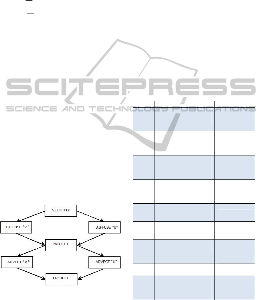
ty in a 3 step process as seen in Figure 1. The diffu-
sion of the densities is first calculated using Equation
1. Then the densities are “moved” by examining the
forces from the vector field and determining their
new locations.
To do this correctly and realistically, the “forc-
es” or the velocity fields must be evolving as well.
The model must create realistic eddies and swirls in
the appropriate places. The process of implementing
this is even more complicated.
The change in the velocity vectors are due to
three main reasons; the addition of forces over time,
the diffusion of the forces and the self-propelling na-
ture of the forces. The diffusion of the forces is cal-
culated similar to the densities, as well as the advec-
tion/movement stage. The new stage is the called the
projection. The projection stage allows for the veloci-
ties to be mass conserving. Additionally, this step
improves the realism of the model by creating eddies
that provide realistic swirling flows.
Figure 1: Velocity Solver steps.
While the framework and execution of the model
may vary from its predecessor, the results are ideally
the same. At the end of every cycle, the densities
have been diffused and moved and the velocity fields
have been updated. The external forces and densities
are added and ready to begin with the next frame.
4 RULES IN Cell-DEVS
A Cell-DEVS model is a lattice of cells holding state
variables and a computing apparatus, which is in
charge of updating the cell states according to a local
rule. This is done using the current cell state and
those of a finite set of nearby cells (called its neigh-
borhood). Cell-DEVS improves execution perfor-
mance of cellular models by using a discrete-event
approach. It also enhances the cell’s timing definition
by making it more expressive. Each cell is defined as
a DEVS atomic model, and it can be later integrated
into a coupled model representing the cell space.
Table 1: Cell Space Layers and Range of Values.
Name Function Values Used
Temp
u
Handles the advection of
"u" component of the ve-
locity vector.
Range: (-2, 2)
Positive = Left
Negative =
Right
Temp
v
Handles the advection of
"v" component. of the ve-
locity vector.
Range: (-2, 2)
Positive = Up
Negative =
Down
U
Handles the final projec-
tion step & stores the fi-
nal values for "u" of the
velocity vectors.
Range: (-2, 2)
Positive = Left
Negative =
Right
V
Handles the final projec-
tion step; stores the final
values for the "v" of the
velocity vectors.
Range: (-2, 2)
Positive = Up
Negative =
Down
Div
Handles the initial projec-
tion step defined as div in
the algorithms
N/A
P
Handles the second pro-
jection step, defined as p
in the algorithms
N/A
Diff'
Handles the diffusion of
the densities
Range: (0, 1)
values in gradi-
ent, 1 = solid &
<1 is a density
Source
Stores densities during
the density calculations
Range: (0, 1)
as above
Final
Handles advection of the
densities and represents
the solution to the density
solver
Range: (0, 1)
as above
Cell-DEVS models in CD++ are built following
the formal specifications of Cell-DEVS and using a
built-in language is provided to describe the behavior
ComputationalFluidDynamicSolverbasedonCellularDiscrete-EventSimulation
219

of each cell. The model specification includes the
definition of the size and dimension of the cell space,
the shape of the neighborhood and borders. The
cell’s local computing function is defined using a set
of rules with the form POSTCONDITION DELAY
{PRE-CONDITION}. These indicate that when the
PRECONDITION is satisfied, the state of the cell
will change to the designated POSTCONDITION,
whose computed values will be transmitted to other
components after consuming the DELAY. If the pre-
condition is false, the next rule in the list is evaluated
until a rule is satisfied or there are no more rules.
Since the cell states are calculated asynchronous-
ly, each cell must contain the following information:
the density of the fluid for that cell space, the veloci-
ty vectors u and v as well as all the intermediate cal-
culations. The cell space will be layered with each
layer holding a different piece of information for its
corresponding cell as shown in Table 1.
Each distinct part of the algorithm, which is de-
fined later, will make use of one or more layers, and
therefore it is very important that the layer infor-
mation be exact.
4.1 Diffusion
The diffusion can be calculated by taking the initial
density value of the cell and adding the scaled sum of
the densities that could enter that cell from the sur-
rounding cells and then calculating the average. The
result is a flow of density from higher to lower con-
centration. By looping this function, we are able to
extend the diffusion to cells outside the neighbor-
hood; however, with a low value for a cell, these val-
ues are negligible at n+/-2 from the cell. The diffu-
sion step is defined with the following equation
(Stam, 2003):
Equation 2 Density Formula
,
,
1,
1,
, 1
, 1
1 4
The implementation of this step is relatively easy.
The values of x are stored in the Source layer and the
values of x' are stored in the Final layer. For each
step the function is run for 20 cycles and on the 20th
cycle the value is stored and the cycle is reset. The
“if” statement in CD++ operates as expected, how-
ever by looking at the timing information we were
able to change its behavior to that of a loop, where
n=20 and after each cycle it restarts at zero. The re-
sulting code looks like the following:
rule:{ if(remainder(time,20)=0,
(0,0,2),(((0,0,2)+0.1*
((1,0,1)+(0,1,1)+(0,1,1)+
(1,0,1)) ))/1.4 ) } 1 { t }
As it can be seen, every time the time variable
reaches a multiple of 20 (i.e. 20 cycles passed)¸ it is
reset. Otherwise, the new density is recalculated
based of the current density, and the weighted aver-
age of the surrounding cells. The amount the average
is weighted is by the variable 'a' which in this situa-
tion is 0.1.
4.2 Advection
The advection step is responsible for the movement
of densities and velocity fields. The most obvious
method of determining where a density will end up is
to trace it forward based on the velocity field. How-
ever, the method described by (Stam, 2003) suggests
starting in the center of the cell space and trace
backwards to find the origins, based on the velocity
field. Then, at this point take the weighted average of
the four closest cells to determine the source density.
This is done because the source will most likely not
fall directly in the middle of the cell and therefore the
surrounding densities would affect the new densities.
The advection step as it appears in the original algo-
rithm is as follows:
void advect ( int N, int b, float *
d, float * d0, float * u, float *
v, float dt ) {
int i, j, i0, j0, i1, j1;
float x, y, s0, t0, s1, t1, dt0;
dt0 = dt*N;
for ( i=1 ; i<=N ; i++ ) {
for ( j=1 ; j<=N ; j++ ) {
x = i-dt0*u[IX(i,j)];
y = j- dt0*v[IX(i,j)];
if (x<0.5) x=0.5;
if (x>N+0.5) x=N+0.5;
i0=(int)x; i1=i0+1;
if (y<0.5) y=0.5;
if (y>N+0.5) y=N+ 0.5;
j0=(int)y; j1=j0+1;
s1 = x-i0; s0 = 1-s1;
t1 = y-j0; t0 = 1-t1;
d[IX(i,j)] = s0*(t0*d0[IX
(i0,j0)]+t1*d0[IX(i0,j1)])
+ s1*(t0*d0[IX(i1,j0)] +
t1*d0[IX(i1,j1)]);
}
}
set_bnd ( N, b, d );
}
This step is used to trace the origins of the current
density by looking at the vector field. Since the
origin is not likely to be at a cell center a weighted
SIMULTECH2013-3rdInternationalConferenceonSimulationandModelingMethodologies,Technologiesand
Applications
220

average of the surrounding four cells is taken, with
their weight dependent on their proximity to the
origin location.
In order to model the advection step is in Cell-
DEVS we are required to include any of the cells
where the density can originate, in the neighborhood.
The first and most important part is ensuring that the
possible source cells are included within the neigh-
borhood. The neighborhood of the advection step is
defined 6 by 6 cells therefore; the maximum distance
a particle can travel is 2 cells from the center. Hence,
the velocity vectors cannot exceed the range of (-
2,2). This can be done by scaling the time step to en-
sure that the velocities remain within the acceptable
limits. For example, if the velocity is 4, it can be
scaled down to 2 and the new time step would be half
of the original. The values of the cells are truncated
to discrete values therefore, there are 5 potential val-
ues: -2,-1,0,1 and 2, for u and v and therefore 25 dif-
ferent combinations of the two. For each combina-
tion, the ratio of the four source cells is calculated.
The following is a portion of the code that deter-
mines the value if the truncated values of the u and v
velocities are 1 and1, respectively.
if( trunc((0,0,-6)) = 1,
if( trunc((0,0,-5)) = 1,
(((1-remainder(abs((0,0,-6)),1))
*((1-remainder(abs((0,0,-5)),1))
*(-1,- 1,-2)+ remainder(
abs((0,0,-5)),1)*(-1,0,-2))+
remainder(abs((0,0,-6)),1)* ((1-
remainder(abs((0,0,-5)),1)) *(0,-1,-
2)+remainder(
abs((0,0,5)),1)*(0,0,-2) )
)
) * this is 1 of 24 possibilities
In this code, it is checking to see if the u and v
vectors fall within the range of 1.0 to 1.999. If this is
the case than by the weighted averages are calculated
and summed.
The code contains 25 iterations of the above code
segment to cover the possible outcomes. This func-
tion is used 3 times in each cycle; the advection of
the density, the advection of u and the advection of v.
However, since the offsets of the required planes are
the same for both u and v (the offset is 0), the func-
tion can be recycled to solve for both. The advection
of the density step, however, requires access to a dif-
ferent plane with a different offset (2) and therefore
must be rewritten with its corresponding neighbor
values.
4.3 Projection
The projection step can be broken into three sub
sections: solving for div, p, u, and v. The original al-
gorithm is implemented using the following code:
void project ( int N, float *u,
float *v, float *p, float *div) {
int i, j, k; float h;
h = 1.0/N;
for ( i=1 ; i<=N ; i++ ) {
for ( j=1 ; j<=N ; j++ ) {
div[IX(i,j)] = -0.5*h*
(u[IX(i+1,j)]- u[IX(i-1,j)]+
v[IX(i,j+1)]-v[IX(i,j-1)]);
p[IX(i,j)] = 0; }
}
set_bnd(N,0,div); set_bnd(N,0,p);
for ( k=0 ; k<20 ; k++ ) {
for ( i=1 ; i<=N ; i++ ) {
for ( j=1 ; j<=N ; j++ ) {
p[IX(i,j)] = (div[IX(i,j)]+
p[IX(i-1,j)]+p[IX(i+1,j)]+
p[IX(i,j-1)]+p[IX(i,j+1)])/4;}
}
set_bnd ( N, 0, p );
}
for ( i=1 ; i<=N ; i++ ) {
for ( j=1 ; j<=N ; j++ ) {
u[IX(i,j)] -= 0.5*(p[IX
(i+1,j)]-p[IX(i-1,j)])/h;
v[IX(i,j)] -= 0.5*(p[IX(i,
j+1)]- p[IX(i,j-1)])/h; }
}
set_bnd(N,1,u); set_bnd ( N, 2, v );
} // (Stam 2003)
The implementation of Div is straightforward. It
takes the two u and two v values from their respec-
tive temp layers and is implemented with the follow-
ing code snippet in CD++ Model file:
rule : { if( remainder( time, 20 ) = 0,
-0.05*((1,0,-4)-(-1,0,-4)+(0,1,-3)
- (0,-1,-3) ), (0,0,0) ) } 1 {t}
As can be seen, the “if” function will work as a
loop that is reset after each iteration. The calculations
are essentially the same with the only difference on
where and how the information is accessed. The -4 at
the end of each neighbor cell means those values are
taken from the temporary layer for the u vectors
while the cells with -3 are taken from the temporary v
vectors.
To solve for p, we use the same method as solv-
ing for the diffusion. The code segment is exactly the
same as mentioned before, however the values of a
are adjusted to reflect the viscosity instead of the dif-
fusion coefficient.
The final step for the projection is the separating
of the vector fields into component form. The sepa-
rating of the horizontal and vertical components in
ComputationalFluidDynamicSolverbasedonCellularDiscrete-EventSimulation
221
our model is performed as it in the algorithm, pre-
sented below:
[u]
rule : { if( remainder(time,20)=0 ,
if( time=0, (0,0,-2),(0,0,-2)-
0.05*((-1,0,-6)-(1,0,-6))),
(0,0,0) ) } 0 { t }
[v]
rule : { if(remainder(time,20) = 0,
if( time = 0, (0,0,-2),
(0,0,-2)-0.05*((0,-1,-7)-
(0,1,-7))),(0,0,0) ) } 0
{t}
During the projection stage, we had added the ve-
locity vectors together to make a single velocity
field. However, for the rest of the algorithm we like
to have the velocities in separate fields. These steps
will be used twice for each cycle of the model.
5 SIMULATION RESULTS
To test the model, we have executed several simula-
tions scenarios. The first simulation was initialized as
single foci of density with the velocity vectors being
randomly generated to have an approximate value of
1, i.e. a velocity in the upwards diagonal to the left.
The diffusion coefficient and the viscosity coefficient
were both set to a low value in the range of (0.1). The
expected result is that the density foci will spread to
more of a cloud with the highest densities being on
the leading edge of the cloud as it proceeds to the top
left corner.
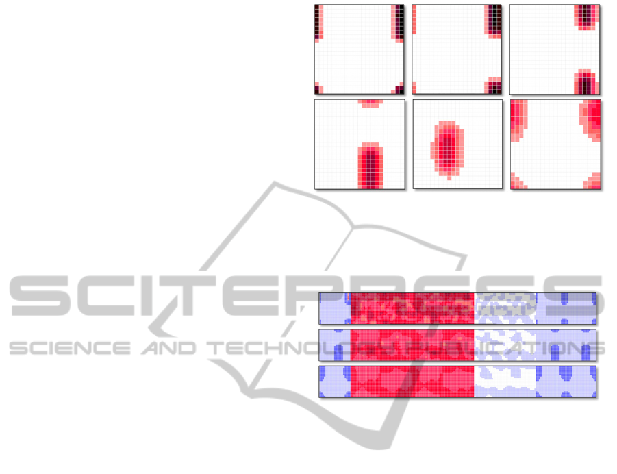
Figure 2 shows the results of simulation scenario
using a cell space of 21 by 21 cells. The coefficient
of diffusion (a) was set to be 0.1. The density field
was exposed to a velocity field whose u and v values
were randomly set to a range of 0.9 to 1. The vis-
cosiy was set as 1. The results illustrated in Figure 2
are what we would expect to see in a real situation.
The density cloud traveled up and left at an angle of
approximately 45 degrees, which corresponds to the
field applied to it. Additionally, the limited disper-
sion of the cloud reflects the low diffusive coefficient
used. The slight teardrop shape that the cloud took
which occurs when the density cloud is moving can
be noticed. The concentration will be slightly higher
on the leading edge and taper out at the end.
Figure 3 demonstrates how over time the velocity
fields become more regular. Since the initial value
assignment was random the field would not be stable.
As the values did not vary too much (max<10%) the
field soon become more evenly distributed and set-
tled between the range of 0.94 to 0.96. This is expec
Figure 2: Progression of Diffusion. Coefficient a= 0.1.
ted since it was a uniform distribution between 0.9
and 1 and with a relatively larger viscosity, the fields
would settle quickly.
Figure 3: Demonstrating the evolving velocity field.
6 CONCLUSIONS
Fluid dynamic solvers are used in a wide variety of
application ranging from video games and entertain-
ment to modeling of environmental events. In this re-
search, a CFD solver is proposed that reuses the pa-
rameters of a CA in Cell-DEVS. The asynchronous
and more efficient computing grid of Cell-DEVS
with the continuous time-base allowed for more real-
istic simulation of the fluid dynamics. We showed
how CD++ toolkit was used to implement the Cell-
DEVS model of the Navier-Stokes equations for
CFD. we were able to create a fluid dynamic solver
that met the requirements of a Cellular Automata,
demonstrating that it is possible to create models of
vary complex phenomenon using a relatively simple
technique. While the model required significantly
longer time to generate results, it provided a more de-
tailed description of what is happening at every stage
of the simulation and stored massive amounts of de-
tail. As an initial implementation, this may not be a
desired characteristic; however such a high level of
detail would allow the model to be integrated easily
to generate a more complex visualization of the fluid
movement.
SIMULTECH2013-3rdInternationalConferenceonSimulationandModelingMethodologies,Technologiesand
Applications
222

REFERENCES
Anderson, J., 2009. Basic philosophy of CFD. In: Compu-
tational Fluid Dynamics. pp. 3-14.
Chen, S. and Doolen. G. 1998. Lattice Boltzman Method
for Fluid Flows. Annual Review of Fluid Mechanics,
Volume 30, pp. 329-364 .
Currie, I. G., 1974. Fundamental Mechanics of Fluids.
McGraw-Hill, Inc.
Frisch U, Hasslacher B, Pomeau Y. 1986. Lattice-gas au-
tomata for the Navier- Stokes equation. Phys Rev Let
56:1505-1508G
Ilachinski, A., 2001. Cellular Automata: A Discrete Uni-
verse. World Scientific Publishing Co.
Koelman, J., 1992. Cellular-Automata-Based Computer
Simulations of Polymer Fluids. Lecture notes in Phys-
ics, Volume 398, pp. 146-153.
Koelman, J. & Nepveu, M., 1992. Darcy flow in porus me-
dia: Cellular Automata Simulations. Lecture notes in
Physics, Volume 398, pp. 136-145.
Saleh, J. M., 2002. Fluid flow handbook. New York:
McGraw-Hill.
Stam, J., 2003. Real-Time Fluid Dynamics for Games.
Proceedings of the Game Developer Conference.
Sukop, M. C. & Thorne, D. T. J., 2006. Lattice Boltzmann
Modeling: An Introduction for Geoscientists and Engi-
neers.:Springer.
Toro, E. F., 2009. Rienmann Solvers and Numerical Meth-
ods for Fluid Dynamics: A Practical Introduction. 3rd
Edition ed. Berlin Heidelberg: Springer-Verlag .
Wainer, G., 2009. Discrete-event modeling and simulation:
a practioner's approach.:CRC.
Zeigler, B. P.; Praehofer, H.; and Kim, Tag-Gon. 2000.
Theory of Modeling and Simulation. Academic Press.
ComputationalFluidDynamicSolverbasedonCellularDiscrete-EventSimulation
223
