Automatic Detection of Single Slow Eye Movements and Analysis of

their Changes at Sleep Onset

Filippo Cona

, Fabio Pizza

, Federica Provini

and Elisa Magosso

Department of Electrical, Electronic and Information Engineering “Guglielmo Marconi”, University of Bologna,

Via Venezia 52, 47521, Cesena, Italy

Department of Biomedical and Neuromotor Sciences, University of Bologna, Bellaria Hospital,

Via Altura 3, 40139, Bologna, Italy

Keywords: Slow Eye Movements, Sleep Onset, Automatic Detection, Template Matching.

Abstract: An algorithm that can automatically identify slow eye movements from the electro-oculogram is presented.

The automatic procedure is trained using the visual classification of an expert scorer. The algorithm makes

use of both the spectral and morphological signal information to detect single slow eye movements. On the

basis of this detection some parameters that characterize the slow eye movements (amplitude, duration,

velocity and number) are extracted. A few possible applications of the algorithm are shown by means of a

preliminary study: the average patterns of slow eye movements parameters at sleep onset are evaluated for

healthy volunteers and for patients affected by obstructive sleep apnea syndrome. Finally, general

considerations are drawn regarding the clinical interest of the study.

1 INTRODUCTION

Eye movements – controlled by a wide neural

network involving the cerebellum, brain stem and

cerebral cortex – may convey important information

on the state and activity of the central nervous

system. Eye movements vary from wakefulness to

sleep and during the different sleep stages. Since

1968, with the recommendation for visual sleep

scoring (Rechtschaffen and Kales, 1968), inspection

of eye movements in electro-oculogram (EOG) is

routinely performed in clinical polysomnography

(PSG) to increase the accuracy and reliability of

sleep stage categorization.

In this work we focus on slow eye movements

(SEMs), which are pendular, predominantly

horizontal eye movements (Aserinsky and Kleitman,

1955); (Värri et al., 1996). SEMs are characteristic

of drowsy wakefulness and light sleep (stages 1 and

2), and occur at the beginning and end of sleep

(Aserinsky and Kleitman, 1955). In recent years,

rising attention has been devoted to SEMs. First,

SEM activity at sleep onset has been investigated in

relation to other physiological and behavioural

measures in order to shed light on the mechanisms

underlying wake-sleep transition (Santamaria and

Chiappa, 1987); (Ogilvie et al., 1988); (De Gennaro

et al., 2000). Furthermore, several studies have

specifically investigated SEMs with the aim of

identifying early predictor of sleep onset to be used

in clinical and occupational settings (Torsvall and

Akerstedt, 1987); (Torsvall and Akerstedt, 1988);

(Marzano et al., 2007).

The growing interest in SEMs has led to

development of various algorithms for automated

SEMs detection in EOG, based on different

techniques and with different aims. However, some

of these algorithms do not identify single SEMs

(Värri et al., 1995); (Virkkala et al., 2007); others

identify single SEMs, but the validation procedure

either exhibits moderate performance (48%

sensitivity) (Värri et al., 1996), or is not examined in

depth (consisting only in the autodetection/visual

scoring ratio) (Hiroshige, 1999); (Suzuki et al.,

2001), or is absent (Shin et al., 2011). Moreover, so

far none of these studies has characterized SEMs in

terms of their parameters (such as amplitude or

duration) nor has investigated how SEMs parameters

evolve across the sleep onset period.

In recent years, we developed an automatic

method for off-line detection of SEM activity in

EOG. The method is based on the wavelet transform

of two unipolar EOG channels; SEM activity is

identified on the basis of EOG power redistribution

474

Cona F., Pizza F., Provini F. and Magosso E..

Automatic Detection of Single Slow Eye Movements and Analysis of their Changes at Sleep Onset.

DOI: 10.5220/0004551304740481

In Proceedings of the 5th International Joint Conference on Computational Intelligence (NCTA-2013), pages 474-481

ISBN: 978-989-8565-77-8

 2013 SCITEPRESS (Science and Technology Publications, Lda.)

towards higher scales (i.e. lower frequencies) of

wavelet decomposition (Magosso et al., 2006). The

method was validated against visual scoring on both

8 h and 24 h PSG recordings acquired in a

laboratory setting (Magosso et al., 2006); (Magosso

et al., 2007); (Magosso et al., 2009). The automatic

method for detection of SEM activity was proven to

perform reliably in detecting sleep onset in

obstructive sleep apnea syndrome (OSAS) patients

(Fabbri et al., 2009); (Fabbri et al., 2010). In a

further study (Pizza et al., 2011), the algorithm was

applied to quantify SEMs distribution during the

different sleep stages and across the sleep cycle.

Despite the promising applications of this

method, it suffers from some drawbacks that may

limit its future use. The main weakness is that the

method was conceived, developed and trained to

detect SEM activity periods – that may consist of an

isolated SEM, a few consecutive SEMs or a long

burst of consecutive SEMs – identifying the initial

and final instants of each period, but without

distinguishing the single eye movements within each

SEM period. Hence, the method is not suitable to

count the number of single SEMs, nor to extract

parameters characterizing each single SEM.

The aim of the present work is to present an

advanced version of the algorithm that overcomes

the previous limitations and a potential application

with some preliminary results. In particular, the new

version of the algorithm improves the previous one

as to the following points: i) it allows the detection

of single slow eye movements in the EOG,

segmenting each identified SEM activity period into

single movements; ii) more importantly, it is able to

extract parameters characterizing each detected slow

eye movement.

The proposed algorithm, being able to extract

and quantify the parameters of SEMs, may have

important clinical implications. In particular,

determination of SEMs parameters (number,

amplitude, duration, velocity) and analysis of their

evolution at the wake-sleep transition may be of

value to characterize – by means of quantitative and

objective measures – the process of falling asleep in

normal, healthy sleepers. This may contribute to a

better description and comprehension of the

complex process of falling asleep. Moreover, the

algorithm can be used to investigate abnormalities of

SEMs parameters in patients suffering from sleep-

related disorders (such as insomnia, OSAS,

narcolepsy), in order to identify potential different

SEMs signatures related to different pathologies,

which may be of clinical significance. In this regard,

the algorithm has been used to assess the evolution

of SEM parameters (amplitude, duration, velocity,

number) at the wake-sleep transition in healthy

volunteers and in OSAS patients, and the obtained

results are critically discussed.

2 METHOD

The new version of the algorithm consists of two

steps. In the first step, the algorithm identifies SEM

activity periods in the EOG: the original version of

the algorithm (Magosso et al., 2006), based on EOG

wavelet decomposition, has been refined in order to

improve its performances. In the second step, the

algorithm segments each identified SEM period into

single SEMs and extracts some fundamental

parameters from the detected movements. The

algorithm was trained and validated on the basis of

visual identification of SEMs performed by a sleep

medicine expert on EOG tracings.

2.1 Data Acquisition

12 healthy subjects and 8 OSAS patients participated

in the study. All subjects gave their written informed

consent for participation in the study which was

conducted with the approval of the local Ethics

Committee. The study consisted in a 24 hours PSG

recording performed in real-life conditions with a

portable digital polygraph (Trex by XLTeck).

Volunteers and patients came to the laboratory for

about 2 hours in the early morning for device

setting, then they left the laboratory, performed their

normal life activities for 24 hours and slept at home.

The next morning returned to the laboratory for

device removing. Recordings included three EEG

derivations (F3-A2, C3-A2, O1-A2; filters: 0.5-70

Hz), one submentalis EMG (filters: 30-100 Hz), two

EOG derivations (E1-A1, E2-A2; filters: 0.1-15 Hz),

and one ECG derivation (filters 1-70 Hz). Each

recording was scored by an expert for sleep staging,

according to the standard visual criteria

(Rechtschaffen and Kales, 1968). Stages were

evaluated in 30-s epochs and labeled as wakefulness

(W) or as one of the five sleep stages (1, 2, 3, 4

NREM, and REM). Signals are sampled at 512 Hz

and resampled at 64 Hz before the processing.

2.2 Visual SEM Scoring

An expert scorer recognized the SEMs on the EOG

traces, in particular in a time window around the

sleep onset (from 15 minutes before stage 1 to 10

minutes after the beginning of stage 2) and the

awakening (from 10 minutes before the end of stage

AutomaticDetectionofSingleSlowEyeMovementsandAnalysisoftheirChangesatSleepOnset

475

2 to 20 minutes after the first wake epoch), since

these are the moments in which the SEMs are more

frequent and distinguishable from other

superimposed activity.

An eye movement was identified as an SEM by

the expert if it met the following criteria: i) single

period of an almost sinusoidal excursion (0.1–1 Hz),

beginning and ending at near-zero velocity; (ii)

amplitude between 20 and 200 µV; (iii) binocular

synchrony with opposed-phase deflections in the

two channels; (iv) onsets of the right and left eye

movement occur within 300 ms of one another; (v)

absence of artefacts (such as blinks, EEG/EMG

artefacts). All the parts of the examined EOG

portions not identified as SEMs, were defined as

Non-SEM (NSEM) activity.

2.3 Identification of SEM Epochs

Following visual detection of single SEMs, the

inspected EOG traces were split into 0.5 s epochs:

one epoch was defined as an SEM epoch according

to the visual classification if at least 50% of the

epoch was covered by an SEM marked by the

expert; otherwise it was classified as an NSEM

epoch. On the basis of this classification we trained

a classifier that categorizes each 0.5 s epoch of EOG

as belonging to SEM or NSEM periods.

To this end, we calculated the discrete wavelet

transform of ΔEOG(t) = EOG

(t) - EOG

(t) (eye

movements give opposite contributions to the two

electrodes) using Daubechies order 4 as wavelet

function, and evaluated 8 scales that approximately

cover the frequency bands 16-32 Hz, 8-16 Hz, 4-8

Hz, 2-4 Hz, 1-2 Hz, 0.5-1 Hz, 0.25-0.5 Hz and

0.125-0.25 Hz respectively. From the wavelet

coefficients we generated another set of 8 time series

pc(t) = [pc(1,t),…,pc(8,t)]: in particular we

performed the principal component analysis (PCA)

of the logarithm to base 10 of the squared wavelet

coefficients. The aim of this processing is to extract

power measures, to make their distribution “more

normal” and then make them uncorrelated through a

change in coordinates.

The 8 quantities pc(n,t) (n = 1,…,8) are

resampled with a time resolution of 0.5 s and

represent the features used in the classifier. Using

the classification of the human scorer we have

generated the distributions P

n,SEM

(pc(n,t)) and

n,NSEM

(pc(n,t)) that represent the probability that a

given value of pc(n,t) is observed during SEM and

NSEM epochs, respectively. As the features are

continuous quantities, the range covering the 98% of

each feature distribution was uniformly divided into

20 bins. Figure 1 shows the frequency distributions

of the features on visually classified SEM and

NSEM epochs (in grey and black respectively).

Figure 1: Distributions P

n,SEM

(pc(n,t)) in gray and

n,NSEM

(pc(n,t)) in black.

The information carried by the 8 values of pc(t)

is then composed into two functions

SEM





 P

,

pc



n,t









(1)

NSEM





 P

,

pc



n,t









(2)

that represent the likelihood that an EOG epoch at

the time t belongs to an SEM or NSEM period

respectively. So the EOG epoch at time t is

classified as an SEM epoch if SEM(t) > NSEM(t),

and as an NSEM epoch otherwise.

The final outcome of this first step is the

identification of SEM activity periods in the EOG

consisting of a single SEM epoch or consecutive

SEM epochs. This first step of the algorithm may be

viewed as a refinement of the algorithm previously

developed and validated by Magosso and colleagues

(Magosso et al., 2006); (Magosso et al., 2007).

Indeed, that algorithm was tested only on EOG

recorded in clinical settings and showed reduced

-5 0 5

0.2

0.4

1,SEM

and P

1,NSEM

pc(1,t)

-2 0 2 4

0.5

2,SEM

and P

2,NSEM

pc(2,t)

-2 0 2

0.5

3,SEM

and P

3,NSEM

pc(3,t)

-1 0 1

4,SEM

and P

4,NSEM

pc(4,t)

-0.5 0 0.5 1

5,SEM

and P

5,NSEM

pc(5,t)

-0.5 0 0.5

6,SEM

and P

6,NSEM

pc(6,t)

-0.5 0 0.5 1

7,SEM

and P

7,NSEM

pc(7,t)

-0.4-0.2 0 0.2 0.4

8,SEM

and P

8,NSEM

pc(8,t)

IJCCI2013-InternationalJointConferenceonComputationalIntelligence

476

performances (results not presented) on EOG

acquired in real-life environments.

2.4 Identification of Single SEMs

The next step of the algorithm is devoted to obtain

an ideal prototype waveform of SEM, φ(t), to be

used as a template to detect single SEMs in each

SEM period identified according to the previous

step. To generate the SEM prototype all the SEMs

identified by the experts have been preprocessed by

i) removing biases and slow trends; ii) normalizing

them in time (all SEMs have been interpolated to

have the same number of time samples) and in

amplitude (each SEM has been divided by its

standard deviation). In this way, only morphological

information is left (figure 2). The generation of this

prototype corresponds to training the algorithm for

the identification of single SEMs.

Figure 2: SEM prototype. The grayscale image on the

background represents the overall distribution of all the

visually scored SEMs (some example are drawn in gray),

while the black plot represents their mean, φ(t).

To identify the single SEMs, we implemented an

“SEM transform” which is very similar to a

continuous wavelet transform, in which the wavelet

function is φ(t). The wavelet functions at different

scales have been obtained by resampling φ(t): for

each length L (in samples) spanning from the

shortest to the longest SEM classified by the expert

min

< L < L

max

) we have created a φ

(k), where

k∈



1,…,L



is the resampling index. After the

resampling, φ

(k) is treated as if it had the same

sampling time as the EOG signal, so the smaller L

the smaller the scale of φ

(k).

For each SEM period identified in the first step,

we can evaluate the correlation coefficient between

the EOG differential mode and each φ

(k), thus

obtaining a map of similarity in the time-scale

domain. In particular, we computed the correlation

coefficient ρ(L,i) between each φ

(k) and

ΔEOG(i+k-L/2)



L,i







L,i





∑

∆EOG



ik

∙





∑











(3)



L,i



  ∆EOGik

∙φ











(4)

where c(L,i) represents the correlation. ρ(L,i) has

values between -1 and 1, where ±1 indicate perfect

match (the concavity of the SEM is not relevant),

while 0 indicates complete uncorrelation. A high

value of |ρ(L,i)| suggests the presence of an SEM

that begins at the time index i-L/2 and ends at time

index i+L/2.

Then a path of points (L

) is found along this

map - where each i

corresponds to the centre of a

SEM of length L

- that satisfies the following

conditions: i) the mean of ρ(L

) is maximized; ii)

each SEM begins within half second the end of the

previous one; iii) the union of all of these SEMs

covers completely the SEM period analysed. For the

sake of brevity, we will not discuss here the

procedure to find the best path that we used in

particular, but any optimization algorithm can

reasonably work.

At the end of this procedure, each SEM period is

subdivided into single SEMs of length L

and

centred in i

. An example of application is illustrated

in figure 3. A 45 s portion of the EOG was

recognized by the algorithm as belonging to a SEM

period; the SEM period was fragmented into single

SEMs on the basis of the similarity with the SEM

prototype at different scales and time shifts.

Note that for each of these SEMs, we can easily

derive the peak-to-peak amplitude in µV, which is

proportional to the correlation c(L

), and the

duration in seconds, which is proportional to L

2.5 SEMs Parameters Extraction

The present algorithm, being able to identify single

SEMs, can extract parameters that characterize the

SEM activity. In this work we focused on the

amplitude, duration, velocity and the number of the

identified SEMs. The algorithm automatically

supplies the amplitude and the duration, while the

other two parameters can be easily derived.

The n

SEM detected by the algorithm, of length

and centred in i

, can be modelled as







c











ki





(5)

(see for example the panel c of figure 3). It is worth

noting that φ

fit

(k) fits the differential EOG.

0 0.2 0.4 0.6 0.8 1

-4

-3

-2

-1

SEM prototype

time (normalized)

amp

(

norma

AutomaticDetectionofSingleSlowEyeMovementsandAnalysisoftheirChangesatSleepOnset

477

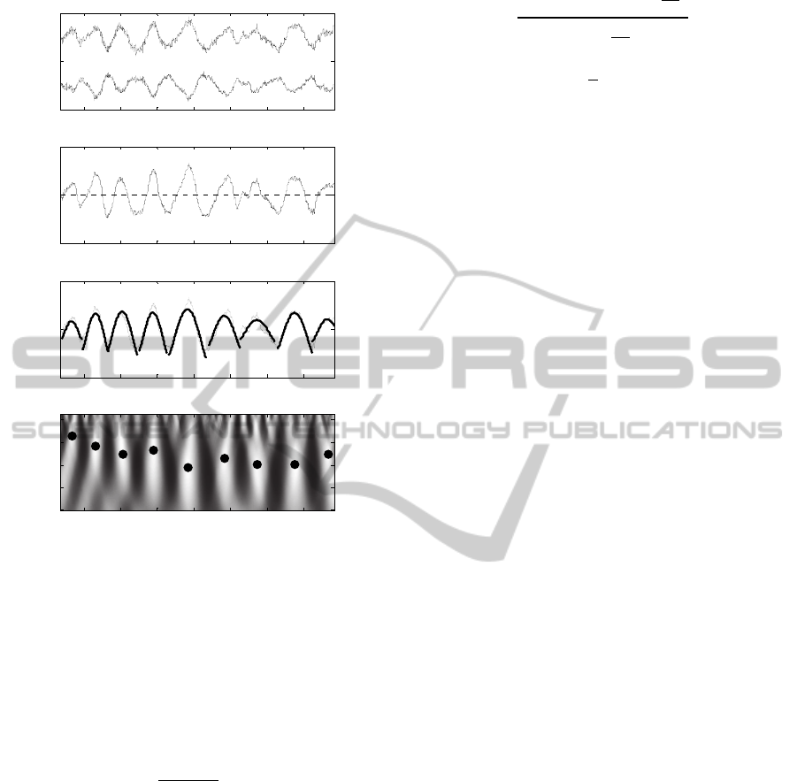
Figure 3: Example of detection of single SEMs in a 45 s

EOG trace. Panel a shows the 2 EOG channels; panel b

shows the differential mode ΔEOG(t); panel c shows the

recognized SEM superimposed to ΔEOG(t); panel d shows

the scale frequency map of the correlation coefficient

ρ(L,i); the black dots indicate the coordinate (L

) of the

SEMs detected.

The amplitude (Amp) in μV and duration (Dur)

in seconds of the SEM are computed as follows:

Amp G







(6)

DurL



⋅Δt

(7)

where G is the ratio between the peak-to-peak

amplitude and the standard deviation of φ(t), and Δt

is the sampling period of the EOG signal (= 1/64 s).

In amplitude computation, the correlation value has

been divided by 2, to obtain measures relative to the

single EOG channels, rather than their difference

(during SEMs the EOG channels have opposite

phases, so ΔEOG(t) has double amplitude with

respect to the single channels).

The velocity (expressed in μV/s) is taken as the

highest mean velocity of the waveform from its

beginning, according to the following formulas:

max









φ



i









ki







⋅Δt

(8)

Vel

(9)

where i

–L

/2 is the initial time index of the

analysed SEM and k is a general time index. As in

amplitude computation, the quantity v is divided by

2, to obtain a measure relative to the single EOG

channels.

Finally, we consider the number (Num) of SEMs

that are recognized in a given time window (e.g. in

Sections 3.2 and 3.3 we will consider 5 minutes time

windows, so Num will be a measure of frequency of

SEMs detected).

A calibration procedure was used to express the

values of the SEM amplitude (Amp) in deg and the

values of the SEM velocity (Vel) in deg/s.

3 RESULTS

In this section, we briefly present the algorithm

performances vs visual scoring. Then we show some

results on SEMs parameters evolution in a time

window around the sleep onset of the healthy

subjects. Finally, the values obtained for healthy

subjects are compared with those obtained for OSAS

patients. Implications of these differences will be

discussed in the Conclusions.

3.1 Validation

A leave one out cross validation has been performed

to assess the performances of the algorithm: all the

subjects but one were used to estimate the

distributions P

n,SEM

(pc(n,t)) and P

n,NSEM

(pc(n,t)) of

SEM and NSEM epochs and to construct the SEM

prototype; then, the distributions and the prototype

φ(t) were used to segment SEMs on the remaining

subject. The procedure has been applied 20 times,

once for each subject. The performances in the

identification of SEM epochs have been assessed in

terms of sensitivity (78.1%) and specificity (87.8%).

As to identification of single SEMs, only the

sensitivity was evaluated (86.0%); the specificity

could not be evaluated since the NSEM epochs are

not subdivided into single eye movements.

3.2 SEMs Parameters Pattern at Sleep

Onset: Healthy Subjects

We analysed the parameters characterizing SEM

927.4 927.5 927.6 927.7 927.8 927.9 928

-200

200

Identification of single SEMs within an SEM period

EOG channels (



927.4 927.5 927.6 927.7 927.8 927.9 928

-200

200



EOG (



time

(

min

)

duration (s)

927.4 927.5 927.6 927.7 927.8 927.9 928

-200

200



EOG (



IJCCI2013-InternationalJointConferenceonComputationalIntelligence

478

activity (extracted as described in 2.5) to describe

how they evolve during the transition from

wakefulness to sleep in healthy subjects.

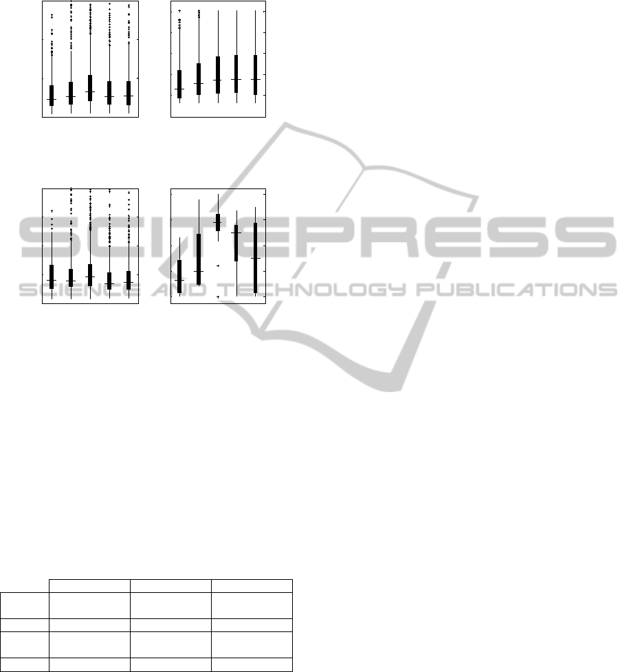
Figure 4: SEM parameters around the sleep onset for the

healthy subjects. Panels a, b, c and d show the

distributions of the values of Amp, Dur, Vel, and Num in

5 time windows of 5 minutes each.

For each healthy subject, we gathered the values

of SEM amplitude (Amp), duration (Dur), velocity

(Vel) and number (Num) of the automatically

identified SEMs during all the wake-sleep

transitions. More specifically, for each transition the

time interval from 12.5 min before to 12.5 min after

the beginning of stage 2 sleep (first epoch of stage 2

sleep) was considered, and all the wake-sleep

transitions occurring in the subjects were aligned to

stage 2 onset. The 25 minutes period at the wake-

sleep transition was subdivided into 5 bins of 5 min

each; all the values of Amp, Dur, Vel and Num of

the SEMs occurring in each bin were collected.

Then, we have generated 5 distributions for each

parameter (one per bin); each distribution is

represented by a boxplot (figure 4). Each panel in

the figure describes the evolution of the parameter

distribution in all the recorded wake-sleep

transitions. As shown in figure 4, SEMs amplitude

(Amp) has a tendency to grow before the beginning

of stage 2, and to decrease afterwards; on the

contrary, SEMs duration (Dur) keeps on increasing

as sleep deepens. Accordingly, SEMs velocity (Vel)

tends to increase before the stage 2 onset, begins to

decrease before the beginning of stage 2 and keeps

on decreasing afterwards. Finally, as shown by the

evolution of Num, SEMs become denser as stage 2

sleep approaches, and gradually become less

frequent as sleep further deepens.

To test the significance of these changes we have

used a Mann-Whitney U-test to compare the

distributions of the parameters between different

time bins. In particular, for each parameter, we

compared the first bin (-10 min) with the second (-5

min) to assess early changes, the second bin with the

third (0 min) to assess changes just before the

beginning of stage 2, and the third bin with the last

(+10 min) to assess changes that take place as sleep

deepens. The amplitude increases significantly

several minutes before stage 2 (from -10 to -5 min)

and decreases significantly during sleep (from 0 to

10 min). The duration significantly increases later

with respect to the amplitude (from -5 to 0 min)

while during the sleep it increases by a non-

significant amount. Velocity, which is proportional

to amplitude and inversely proportional to duration,

behaves accordingly: it increases significantly from -

10 to -5 minutes and decreases significantly both

from -5 to 0 minutes and from 0 to 10 minutes. The

number of SEMs also changes significantly on the

whole 25 minutes of analysis: it increases before

stage 2 and decreases afterwards. The p-values,

corrected with Bonferroni correction (24

comparisons, 12 for healthy subjects and 12 for

OSAS patients), are given in table 1.

Table 1: p-Values of the statistical analysis for the healthy

subjects.

-10 Vs. -5 -5 Vs. 0 0 Vs. 10

Amp

2.93e-8

***

5.71

6.32e-10

***

Dur 9.40

1.58e-7

***

2.71

Vel

4.14e-9

***

6.32e-7

***

4.53e-15

***

Num

2.20e-3

7.20e-3

1.01e-4

***

3.3 SEMs Parameters Pattern at Sleep

Onset: OSAS Patients

The same analysis has been performed for the OSAS

patients (figure 5). The results suggest that the

parameters for this second category of subjects have

less significant excursions. Before the sleep, the

increase in amplitude is delayed with respect to

healthy subjects, becoming significant from -5 to 0

min, rather than from -10 to -5, and the p-values are

-10 -5 0 5 10

time to stage 2 (min)

Amplit ude ( °)

-10 -5 0 5 10

time to stage 2 (min)

Duration (s)

-10 -5 0 5 10

time to stage 2 (min)

Veloc ity ( °/s )

-10 -5 0 5 10

time to stage 2 (min)

Number of SEMs

AutomaticDetectionofSingleSlowEyeMovementsandAnalysisoftheirChangesatSleepOnset

479

globally larger. The duration increases continuously

but always by a non-significant amount.

Figure 5: SEM parameters around the sleep onset for the

OSAS patients. The panels show the same measures as

those of figure 4.

The velocity has a completely different evolution

in OSAS patients, since in the second bin it totally

lacks the very high values that are observed in

healthy subjects. Finally, the number of SEMs

follows qualitatively the same evolution as for the

healthy subjects, but the changes are not significant.

The p-values, corrected with Bonferroni correction

(see 3.2), are given in table 2.

Table 2: p-values of the statistical analysis for the OSAS

patients.

-10 Vs. -5 -5 Vs. 0 0 Vs. 10

Amp 6.22e-1

2.49e-4

***

8.39e-5

***

Dur 7.99e-2 1.95e-1 16.6

Vel 23.9

2.69e-2

1.59e-9

***

Num 8.85e-1 8.11e-1 6.30e-1

4 CONCLUSIONS

In this work we have presented an algorithm for

SEM detection which represents a substantial

improvement of our previous version (Magosso et

al., 2006; Magosso et al., 2007). Whereas the latter

was able to merely detect periods of SEM activity,

without segmenting single SEMs, the new algorithm

takes advantage of spectral and morphological

information to automatically detect single SEMs in

EOG, showing high performances vs. visual scoring.

Hence, the algorithm is able to count the single

SEMs that occurred in a given time window;

furthermore, and of great relevancy, the algorithm

extracts specific parameters from each recognized

SEM, in particular amplitude, velocity and duration.

These new features of the algorithm open

important perspectives for basic and clinical

research. As SEMs are a phenomenon typical of the

sleep onset period, quantification of SEMs

parameters and analysis of their evolution at the

wake-sleep transition can contribute to improve the

understanding of the process of falling asleep.

Indeed, this process - although widely investigated -

is still far from being fully understood and its

comprehension can benefit from a more precise

depiction of oculomotor changes. Furthermore, the

algorithm may be a valid tool to detect potential

modifications of SEMs parameters at sleep onset in

patients suffering from sleep-related disorders

(insomnia, narcolepsy, OSAS) compared to normal

sleepers, thus characterizing abnormalities in the

process of falling asleep via quantitative measures

provided by SEMs behavior. Regarding to this point,

this paper presents some preliminary results

obtained on a limited number of subjects. In

particular, SEMs parameters in the healthy subjects

and OSAS patients seem to exhibit different

evolutions at the sleep onset period. On average, in

healthy subjects, SEMs parameters change clearly:

they increase in number, amplitude and velocity

before stage 2 onset; afterwards, SEMs rapidly

decrease in number, and change their morphology

flattening and lengthening. On the contrary, in

OSAS patients, SEMs parameters change by a less

amount, exhibiting on the overall a flatter pattern

across the five temporal bins that cover the sleep

onset period. The obtained results suggest that SEMs

might signal differences in the process of falling

asleep in the patients compared to normal. The

healthy volunteers fall asleep starting from relaxed

vigilance state that consists of a few epochs of stage

1 sleep followed by stage 2 sleep and deeper stages

later on. On the other hand, the OSAS patients fall

asleep with a longer, uneven pattern of vigilance

states and they are more prone to wake up from

stage 1 and even stage 2 sleep. The absence of a

definite evolution of SEMs parameters in OSAS

patients could be a marker of the pathological route

into sleep. However, it is worth noticing that this

-10 -5 0 5 10

time to stage 2 (min)

Amplitude (°)

-10 -5 0 5 10

time to stage 2 (min)

Duration (s)

-10 -5 0 5 10

time to stage 2 (min)

Velocity (°/s)

-10 -5 0 5 10

time to stage 2 (min)

Number of SEMs

IJCCI2013-InternationalJointConferenceonComputationalIntelligence

480

interpretation is far from being conclusive especially

because of the reduced size of the OSAS sample;

further and deeper analyses with a higher number of

subjects are mandatory to confirm these results and

eventually disclose other potential explanations.

In future, the algorithm will also be applied to

patients suffering from other sleep-related

disturbances to provide a depiction of the SEMs

signatures in different pathologies.

ACKNOWLEDGEMENTS

This work has been supported by a National project

funded by the Italian Ministry for the Environment,

Land and Sea “Excessive daytime drowsiness and

road accidents: Specific risks in the transportation

of waste and toxic harmful substances of significant

ecological impact.”

REFERENCES

Aserinsky, E. and Kleitman, N. (1955). Two types of

ocular motility occurring in sleep. Journal of Applied

Physiology, 8(1), pp.1–10.

Fabbri, M., Pizza, F., Magosso, E., Ursino, M., Contardi,

S., Cirignotta, F., Provini, F. and Montagna, P. (2010).

Automatic slow eye movement (SEM) detection of

sleep onset in patients with obstructive sleep apnea

syndrome (OSAS): comparison between multiple

sleep latency test (MSLT) and maintenance of

wakefulness test (MWT). Sleep Medicine, 11(3),

pp.253–257.

Fabbri, M., Provini, F., Magosso, E., Zaniboni, A., Bisulli,

A., Plazzi, G., Ursino, M. and Montagna, P. (2009).

Detection of sleep onset by analysis of slow eye

movements: a preliminary study of MSLT recordings.

Sleep Medicine, 10(6), pp.637–640.

De Gennaro, L., Ferrara, M., Ferlazzo, F. and Bertini, M.

(2000). Slow eye movements and EEG power spectra

during wake-sleep transition. Clinical

Neurophysiology, 111(12), pp.2107–2115.

Hiroshige, Y. (1999). Linear automatic detection of eye

movements during the transition between wake and

sleep. Psychiatry and Clinical Neurosciences, 53(2),

pp.179–181.

Magosso, E., Provini, F., Montagna, P. and Ursino, M.

(2006). A wavelet based method for automatic

detection of slow eye movements: a pilot study.

Medical Engineering & Physics, 28(9), pp.860–875.

Magosso, E., Ursino, M., Zaniboni, A. and Gardella, E.

(2009). A wavelet-based energetic approach for the

analysis of biomedical signals: Application to the

electroencephalogram and electro-oculogram. Applied

Mathematics and Computation, 207(1), pp.42–62.

Magosso, E., Ursino, M., Zaniboni, A., Provini, F. and

Montagna, P. (2007). Visual and computer-based

detection of slow eye movements in overnight and 24-

h EOG recordings. Clinical Neurophysiology, 118(5),

pp.1122–1133.

Marzano, C., Fratello, F., Moroni, F., Pellicciari, M.,

Curcio, G., Ferrara, M., Ferlazzo, F. and De Gennaro,

L. (2007). Slow eye movements and subjective

estimates of sleepiness predict EEG power changes

during sleep deprivation. Sleep, 30(5), pp.610–616.

Ogilvie, R.D., McDonagh, D.M., Stone, S.N. and

Wilkinson, R.T. (1988). Eye movements and the

detection of sleep onset. Psychophysiology, 25(1),

pp.81–91.

Pizza, F., Fabbri, M., Magosso, E., Ursino, M., Provini, F.,

Ferri, R. and Montagna, P. (2011). Slow eye

movements distribution during nocturnal sleep.

Clinical Neurophysiology, 122(8), pp.1556–1561.

Rechtschaffen, A. and Kales, A. (1968). A manual of

standardized terminology, techniques and scoring

system of sleep stages in human subjects. Los Angeles,

UCLA.

Santamaria, J. and Chiappa, K.H. (1987). The EEG of

drowsiness in normal adults. Journal of Clinical

Neurophysiology, 4(4), pp.327–382.

Shin, D., Sakai, H. and Uchiyama, Y. (2011). Slow eye

movement detection can prevent sleep-related

accidents effectively in a simulated driving task.

Journal of Sleep Research, 20(3), pp.416–424.

Suzuki, H., Matsuura, M., Moriguchi, K., Kojima, T.,

Hiroshige, Y., Matsuda, T. and Noda, Y. (2001). Two

auto-detection methods for eye movements during

eyes closed. Psychiatry and Clinical Neurosciences,

55(3), pp.197–198.

Torsvall, L. and Akerstedt, T. (1988). Extreme sleepiness:

quantification of EOG and spectral EEG parameters.

The International Journal of Neuroscience, 38(3-4),

pp.435–441.

Torsvall, L. and Akerstedt, T. (1987). Sleepiness on the

job: continuously measured EEG changes in train

drivers. Electroencephalography and Clinical

Neurophysiology, 66(6), pp.502–511.

Värri, A., Hirvonen, K., Häkkinen, V., Hasan, J. and

Loula, P. (1996). Nonlinear eye movement detection

method for drowsiness studies. International Journal

of Bio-Medical Computing, 43(3), pp.227–242.

Värri, A., Kemp, B., Rosa, A.C., Nielsen, K.D., Gade, J.,

Penzel, T., Hasan, J., Hirvonen, K., Häkkinen, V.,

Kamphuisen, H.A.C. and Mourtazaev, M.S. (1995).

Multi-centre comparison of five eye movement

detection algorithms. Journal of Sleep Research, 4(2),

pp.119–130.

Virkkala, J., Hasan, J., Värri, A., Himanen, S. and Härmä,

M. (2007). The use of two-channel electro-

oculography in automatic detection of unintentional

sleep onset. Journal of Neuroscience Methods, 163(1),

pp.137–144.

AutomaticDetectionofSingleSlowEyeMovementsandAnalysisoftheirChangesatSleepOnset

481