Feature Selection by Rank Aggregation and Genetic Algorithms

Waad Bouaguel

, Afef Ben Brahim

and Mohamed Limam

1,2

LARODEC, ISGT, University of Tunis, Tunis, Tunisia

Dhofar University, Salalah, Oman

Keywords:

Rank Aggregation, Distance Function, Filter Methods, Feature Selection, Data Dimensionality.

Abstract:

Feature selection consists on selecting relevant features in order to focus the learning search. A simple and

efﬁcient setting for feature selection is to rank the features with respect to their relevance. When several

rankers are applied to the same data set, their outputs are often different. Combining preference lists from

those individual rankers into a single better ranking is known as rank aggregation. In this study, we develop a

method to combine a set of ordered lists of feature based on an optimization function and genetic algorithm.

We compare the performance of the proposed approach to that of well-known methods. Experiments show that

our algorithm improves the prediction accuracy compared to single feature selection algorithms or traditional

rank aggregation techniques.

1 INTRODUCTION

The continued progress in developing different statis-

tical methods focusing on the same research question

have allowed investigating the search for ways to use

various methods simultaneously. To get the best re-

sult of all available alternatives, we need to integrate

their results in an efﬁcient way. In the task of feature

selection, rank aggregation is an example of these in-

tegration methods.

Feature selection is an important stage of prepro-

cessing commonly used in data mining applications,

where a subset of the features that most contribute to

accuracy are selected. Feature selection is also a way

of avoiding the curse of dimensionality which occurs

when the number of availablefeatures signicantly out-

numbers the number of examples, as is the case in Bio

Informatics. Feature selection methods divide into

wrappers, ﬁlters, and embedded methods (Guyon and

Elisseff, 2003). Wrappers employ the learning algo-

rithm of interest as a black box to score subsets of

features according to their predictive power (Kohavi

and John, 1997). Filters select subsets of features as a

pre-processing step, independently of the chosen pre-

dictor. Embedded methods perform feature selection

in the process of training and are usually specic to

given learning algorithms. It is argued that, compared

to wrappers, ﬁlters are faster and that some ﬁlters pro-

vide a generic selection of features, not tuned for a

given learning algorithm. Another advantage of ﬁl-

ters is that they can be used as a preprocessing step to

reduce space dimensionality and overcome overtting

(Guyon and Elisseff, 2003).

A particularly optimal implementation of ﬁlters

are methods that employ some criterion to score each

feature and provide a ranking (Caruana et al., 2003)

(Weston et al., 2003). From this ordering, several fea-

ture subsets can be chosen. This kind of the ﬁlter ap-

proach, that are known as rankers, can be extremely

efﬁcient because they are quite simple. When apply-

ing multiple rankers based on different scoring cri-

teria we have often different feature ranking lists so

ﬁnding a way to aggregate them is required. Rank

aggregation is to combine ranking results of entities

from multiple ranking functions in order to generate a

better one (Borda, 1781) (Dwork et al., 2001).

Most of rank aggregation methods treat all the

ranking lists equally and give high ranks to those enti-

ties ranked high by most of the rankers. This assump-

tion may not hold in practice, however. For example,

for a given problem, a ranking list may give better

classiﬁcation results than the others. It is not reason-

able to treat the results of all ranking lists equally.

To deal with the problem, weighted rank aggre-

gation techniques can be employed where different

rankers are assigned different weights. For example,

the weights can be calculated based on the mean av-

erage precision scores of the base rankers. In this

paper we investigate the use of ranking lists impor-

tance, based on their corresponding classiﬁcation ac-

Bouaguel W., Ben Brahim A. and Limam M..

Feature Selection by Rank Aggregation and Genetic Algorithms.

DOI: 10.5220/0004518700740081

In Proceedings of the International Conference on Knowledge Discovery and Information Retrieval and the International Conference on Knowledge

Management and Information Sharing (KDIR-2013), pages 74-81

ISBN: 978-989-8565-75-4

 2013 SCITEPRESS (Science and Technology Publications, Lda.)

curacy, in addition to feature weights in order to high-

light ranking lists that give better classiﬁcation results

and features that are more relevant than others even

if they are equally ranked by different rankers. These

parameters are used by a genetic algorithm that re-

ceives multiple ranking lists and generate a ﬁnal ro-

bust feature ranking list.

2 RANK AGGREGATION

Feature ranking consists on ranking the features with

respect to their relevance, one selects the top ranked

features, where the number of features to select is

specied by the user or analytically determined.

Many feature selection algorithms include feature

ranking as a principal selection mechanism because of

its simplicity, scalability, and good empirical success.

Several papers in this issue use variable ranking as a

baseline method (Caruana et al., 2003) (Weston et al.,

2003).

Let X a matrix containing m instances x

, . . . , x

) ∈ R

. we denote by y

= (y

, . . . , y

) the

vector of class labels for the m instances. A is the set

of features a

= (a

, . . . , a

Feature ranking makes use of a scoring function

H( j) computed from the values x

and y

. By con-

vention, we assume that a high score is indicative of

a valuable variable and that we sort variables in de-

creasing order of H( j).

Feature ranking is a ﬁlter method thus it is inde-

pendent of the choice of the predictor. Even when

feature ranking is not optimal, it may be preferable

to other feature subset selection methods because of

its computational and statistical scalability: Compu-

tationally, it is efcient since it requires only the com-

putation of d scores and sorting the scores; Statisti-

cally, it is robust against overtting because it intro-

duces bias but it may have considerably less variance

(Hastie et al., 2001).

When applying scoring functions based on differ-

ent scoring criteria we have often different feature

ranking lists so ﬁnding a way to aggregate them is

required. The rank aggregation problem is to com-

bine many different rank orderings on the same set of

candidates, or alternatives, in order to obtain a bet-

ter ordering. This is a classical problem from social

choice and voting theory, in which each voter gives

a preference on a set of alternatives, and the system

outputs a single preference order on the set of alterna-

tives based on the voters’ preferences (Borda, 1781)

(Young, 1990).It is the key problem in many applica-

tions. For example, in sports and competition to rank

or to compare players from different eras. In machine

learning to do collaborative ltering and meta-search;

in database middleware to combine results from mul-

tiple databases. In recent years, rank aggregation

methods have emerged as an important tool for com-

bining information from different Internet search en-

gines or from different omics-scale biological studies

(Dwork et al., 2001). Ordered lists are routinely pro-

duced by today’s high-throughput techniques which

naturally lend themselves to a meta-analysis through

rank aggregation. (DeConde et al., 2006) proposed to

use rank aggregation methods to integrate the results

of several ordered lists of genes.

When aggregating feature rankings, there are two

issues to consider. The ﬁrst one is which base fea-

ture rankings to aggregate. There are different ways

to generate the base feature rankings: the ﬁrst uses

the same dataset, but by different ranking method, the

second one uses different subsamples of the dataset

but the same ranking method. In our experiments we

use the ﬁrst ranking generation technique. The sec-

ond issue concerns the type of aggregation function

to use. There are mainly two kinds of rank aggre-

gation, score-based rank aggregation and order-based

rank aggregation. In the former, objects in the input

rankings are associated with scores, while in the latter,

only the order information of these objects is avail-

able. The Borda count (Borda, 1781) and median

rank aggregation are the most famous such method

where elements in the overall list are ordered accord-

ing to the average rank computed from the ranks in

all individual lists. Another category is based on the

majoritarian principles and attempts to accommodate

the ”majority” of individual preferences putting less

or no weight on the relatively infrequent ones. The

ﬁnal aggregate ranking is usually based on the num-

ber of pairwise wins between items within individ-

ual lists. Any method that satisﬁes this condition,

known as the Condorcet criterion, is called the Con-

dorcet method (Young, 1990) (Young and Levenglick,

1978). In the recent literature, probabilistic models

on permutations, such as the Mallows model and the

Luce model, have been introduced to solve the prob-

lem of rank aggregation. In this work, we take advan-

tage from the two kinds, order-basedrank aggregation

but also score-based rank aggregation in order to not

lose the additional score information.

3 PROPOSED APPROACH

3.1 Optimization Problem

Rank aggregation provides a mean of combining in-

formation from different ordered lists and at the same

FeatureSelectionbyRankAggregationandGeneticAlgorithms

Figure 1: Rank Aggregation.

time, to set their weak points. The aim of rank aggre-

gation when dealing with feature selection is to ﬁnd

the best list, which would be the closest as possible to

all individual ordered lists all together.

This can be seen as an optimization problem,

when we look at argmin(D, σ), where argmin gives

a list σ at which the distance D with a randomly se-

lected ordered list is minimized. In this optimization

framework the objective function is given by :

F(σ) =

∑

i=1

× D(σ, L

), (1)

where w

represent the weights associated with the

lists L

, D is a distance function measuring the dis-

tance between a pair of ordered lists ( for more details

see Section 3.2) and L

is the i

ordered list of cardi-

nality k. The best solution is then to look for σ

∗

which

would minimize the total distance between σ

∗

and L

given by

∗

= argmin

∑

i=1

× D(σ, L

). (2)

3.2 Distance Measures

Measuring the distance between two ranking lists is

classical and several well-studied metrics are known

(Carterette, 2009; Kumar and Vassilvitskii, 2010), in-

cluding the Kendall’s tau distance and the Spearman

footrule distance. Before deﬁning this two distance

measures, let us introduce some necessary notation.

Let S

(1), . . . , S

(k) be the scores coupled with the ele-

ments of the ordered list L

, where S

(1) is associated

with the feature on top of L

that is most important,

and S

(k) is associated with the feature which is at the

bottom that is least important with regard to the target

concept. All the other scores correspond to the fea-

tures that would be in-between, ordered by decreasing

importance.

For each item j ∈ L

, r( j) shows the ranking of this

item. Note that the optimal ranking of any item is 1,

rankings are always positive, and higher rank shows

lower preference in the list.

3.2.1 Spearman Footrule Distance

Spearman footrule distance between two given rank-

ings lists L and σ, is deﬁned as the sum, overall the

absolute differences between the ranks of all unique

elements from both ordered lists combined. Formally,

the Spearman footrule distance between L and σ, is

given by

Spearman(L, σ) =

∑

f∈(L∪σ)

( f) − r

( f)| (3)

Spearman footrule distance is a very simple way for

comparing two ordered lists. The smaller the value of

this distance, the more similar the lists. When the two

lists to be compared, have no elements in common,

the metric is k(k + 1).

3.2.2 Kendall’s Tau Distance

The Kendall’s tau distance between two ordered rank

list L and σ, is given by the number of pairwise ad-

jacent transpositions needed to transform one list into

another (Dinu and Manea, 2006). This distance can

be seen as the number of pairwise disagreements be-

tween the two rankings. Hence, the formal deﬁnition

for the Kendall’s tau distance is:

Kendall(L,σ) =

∑

i, j∈(L∪σ)

K, (4)

where

K =











0 if r

(i) < r

( j), r

(i) < r

( j)

or r

(i) > r

( j), r

(i) > r

( j)

1 if r

(i) > r

( j), r

(i) < r

( j)

or r

(i) < r

( j), r

(i) > r

( j)

p if r

(i) = r

( j) = k + 1,

(i) = r

( j) = k + 1

(5)

That is, if we have no knowledge of the relative

position of i and j in one of the lists, we have sev-

eral choices in the matter. We can either impose

no penalty (0), full penalty (1), or a partial penalty

(0 < p < 1).

3.2.3 Weighted Distance

In case, the only information available about the in-

dividual list is the rank order, the Spearman footrule

distance and the Kendall’s tau distance are adequate

measures. However the presence of any additional

KDIR2013-InternationalConferenceonKnowledgeDiscoveryandInformationRetrieval

information about the individual list may improve

the ﬁnal aggregation. Typically with ﬁlter methods,

weights are assigned to each feature independently

and then the features are ranked based on their rel-

evance to the target variable. It would be beneﬁcial to

integrate these weights into our aggregation scheme.

Hence, the weight associated to each feature consists

of taking the average score across all of the ranked

feature lists. We ﬁnd the average for each feature by

adding all the normalized scores associated to each

lists and dividing the sum by the number of lists.Thus,

the weighted Spearman’s footrule distance between

two list L and σ is given by

∑

f∈(L∪σ)

|W(r

( f)) × r

( f) −W(r

( f)) × r

( f)|.

∑

f∈(L∪σ)

|W(r

( f))−W(r

( f))|×|r

( f)−r

( f)|.

(6)

Analogously to the weighted Spearman’s footrule

distance, the weighted Kendall’s tau distance is given

by:

WK(L, σ) = |W(r

(i)) −W(r

( j))|K. (7)

3.3 Solution to Optimization Problem

Using Genetic Algorithm

The introduced optimization problem in Section 3.1

is a typical integer programming problem. As far as

we know, there is no efﬁcient solution to such kind of

problem. One possible approach would be to perform

complete search. However, it is too time demanding

to make it applicable in real applications. We need to

look for more practical solutions.

The presented method uses a genetic algorithm for

rank aggregation. Genetic algorithms (GAs) were in-

troduced by (Holland, 1992) to imitate the mechanism

of genetic models of natural evolution and selection.

GAs are powerful tools for solving complex for solv-

ing combinatorial problems, where a combinatorial

problem involves choosing the best subset of com-

ponents from a pool of possible components in or-

der that the mixture has some desired quality (Clegg

et al., 2009). GAs are computational models of evo-

lution. They work on the basis of a set of candidate

solutions. Each candidate solution is called a ”chro-

mosome”, and the whole set of solutions is called a

”population”. The algorithm allows movement from

one population of chromosomes to a new population

in an iterative fashion. Each iteration is called a ”gen-

eration”. GAs in our case proceeds in the following

manner :

3.3.1 Initialization

Once a set of aggregation rank lists are generated by

several ﬁltering techniques, it is necessary to create

an initial population of features to be used as starting

point for the genetic algorithm, where each feature

in the population represents a possible solution. This

starting population is then obtained by randomly se-

lecting a set of ordered rank lists.

Despite the success of genetic algorithm on a wide

collection of problems, the choice of the population

size stills an issue. (Gotshall and Rylander, ) proved

that the larger the population size, the better chance of

it containing the optimal solution. However, increas-

ing population size also causes the number of genera-

tions to convergeto increase. In order to havegreat re-

sults, the population size should depend on the length

of the ordered lists and on the number of unique el-

ements in these lists. From empirical studies, over a

wide range of problems, a population size of between

30 and 100 is usually recommended.

3.3.2 Selection

Once the initial population is ﬁxed, we need to select

new members for the next generation. In fact, each el-

ement in the current population is evaluated on the ba-

sis of its overall ﬁtness (the objective function score).

Depending on which distance is used, new members

(rank lists) are produced by selecting high performing

elements (Vafaie and Imam, 1994).

3.3.3 Cross-over

The selected members are then crossed-over with the

cross-over probability CP. Crossover randomly select

a point in two selected lists and exchange the re-

maining segments of these lists to create a new ones.

Therefore, crossover combines the features of two

lists to create two similar ranked lists

3.3.4 Mutation

In case only the crossover operator is used to produce

the new generation, one possible problem that may

arise is that if all the ranked lists in the initial popula-

tion have the same value at a particular rank, then all

future lists will have this same value at this particular

rank. To come over this unwanted situation a muta-

tion operator is used. Mutation operates by randomly

changing one or more elements of any list. It acts as a

population perturbation operator. Typically mutation

does not occur frequently so mutation is of the order

FeatureSelectionbyRankAggregationandGeneticAlgorithms

4 EXPERIMENTAL SETUP

4.1 Datasets

As discussed before using too much data, in terms of

the number of input variables, is not always effective.

This is especially true when the problem involves un-

supervised learning or supervised learning with un-

balanced data (many negative observations but mini-

mal positive observations). This paper addresses two

issues involving high dimensional data: The ﬁrst is-

sue explores the behavior of ensemble method fea-

ture aggregation when analyzing data with hundreds

or thousands of dimensions in small sample size situ-

ations. The second issue deals with huge data set with

a massive number of instances and where feature se-

lection is used to extract meaningful rules from the

available data.

The experiments for the ﬁrst case were conducted

on Central Nervous System (CNS), a large data set

concerned with the prediction of central nervous sys-

tem embryonal tumor outcome based on gene expres-

sion. This data set includes 60 samples containing 39

medulloblastoma survivors and 21 treatment failures.

These samples are described by 7129 genes(Pomeroy

et al., 2002). We consider also the Leukemia mi-

croarry gene expression dataset that consists of 72

samples which are all acute leukemia patients, ei-

ther acute lymphoblastic leukemia (47 ALL) or acute

myelogenous leukemia (25 AML). The total number

of genes to be tested is 7129. (Golub et al., 1999)

For the second case two credit datasets are used,

the German and the Tunisian credit dataset. The Ger-

man credit dataset covers a sample of 1000 credit con-

sumers where 700 instances are creditworthy and 300

are not. For each applicant, 21 numeric input vari-

ables are available .i.e. 7 numerical, 13 categorical

and a target attribute. The Tunisian dataset covers a

sample of 2970 instances of credit consumers where

2523 instances are creditworthy and 446 are not. Each

credit applicant is described by a binary target vari-

able and a set of 22 input variables were 11 features

are numerical and 11 are categorical. Table 2 displays

the characteristics of the datasets that have been used

for evaluation.

Table 1: Datasets summary.

Names German Tunisian CNS Leukemia

Instances 1000 2970 60 72

Features 20 22 7129 7129

Classes 2 2 2 2

Miss-values No Yes No No

4.2 Feature Rankers

We investigated three different ﬁlter selection algo-

rithms from the category of rankers, Relief algorithm

(Kira and Rendell, 1992), Correlation-based feature

selection (CFS) (Hall, 2000) and Information gain

(IG) (Quinlan, 1993). These algorithms are available

in Weka 3.7.0 machine learning package (Bouckaert

et al., 2009).

Relief algorithm evaluates each feature by its abil-

ity to distinguish the neighboring instances. It ran-

domly samples the instances and checks the instances

of the same and different classes that are near to each

other.

Correlation-based Feature Selection (CFS) looks

for feature subsets based on the degree of redundancy

among the features. The objective is to ﬁnd the fea-

ture subsets that are individually highly correlated

with the class but have low inter-correlation. The sub-

set evaluators use a numeric measure, such as con-

ditional entropy, to guide the search iteratively and

add features that have the highest correlation with the

class.

Information gain (IG) measures the number of bits

of information obtained for class prediction by know-

ing the presence or absence of a feature.

4.3 Classiﬁcation Algorithms and

Performance Metrics

We trained our approach using three well-known data

mining algorithms, namely Decision trees, Support

vector machines and The K-nearest-neighbor. These

algorithms are available in Weka 3.7.0 machine learn-

ing package (Bouckaert et al., 2009).

To evaluate the classiﬁcation performance of each

setting and perform comparisons, we used several

characteristics of classiﬁcation performance all de-

rived from the confusion matrix (Okun, 2011). We

deﬁne brieﬂy these evaluation metrics.

The precision is the percentage of positive predic-

tions that are correct. The Recall (or sensitivity) is the

percentage of positive labeled instances that were pre-

dicted as positive. The F-measure can be interpreted

as a weighted average of the precision and recall. It

reaches its best value at 1 and worst score at 0.

The cited performance measures are obtained

when the cut-off is 0.5. However, changing this

threshold might modify previous results. In this pa-

per we use the AUC (the area under the ROC curve)

as graphical tool to evaluate the effect of selected fea-

tures on classiﬁcation models (Ferri et al., 2009).

KDIR2013-InternationalConferenceonKnowledgeDiscoveryandInformationRetrieval

5 RESULTS

Tables 3-5 report on the performances achieved by

DT, SVM and KNN algorithms using the individ-

ual ﬁlters, mean aggregation and genetic algorithm.

In general the discussed feature selection approaches

perform well for selecting relevant features either for

small or high data dimensionality. There is obvi-

ously a strong similarity in the feature sets selected

by different approaches. A more detailed picture of

the achieved results shows that the precision of ag-

gregation approaches is better than most of the stud-

ied ﬁlters. Consistent with the theoretical analysis

for feature selection, the fusion approach usually out-

performs single ﬁlters. However, we should consider

individual results to conﬁrm the superiority of our ap-

proach.

For information ﬁltering as feature selection prob-

lems, one cares the most about both the precision and

the recall of the classiﬁcation using individual and en-

semble feature selection methods. F-measure is the

metric of choice for considering both together.

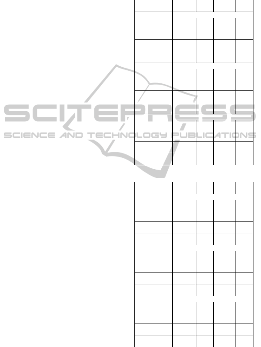
For the German dataset, in all cases the ﬁlters

aggregation gives better performance than individual

feature selection methods. For DT, the genetic al-

gorithm (GA) both with Kendall and Spearman dis-

tances gives better results than the mean aggregation

technique but it is not always true when taking ROC

area as a performance metric.

The outperformance of GA is also noticeable for

KNN classiﬁer when comparing recall and F-measure

performance metrics. However for SVM classiﬁer,

mean aggregation gives better results than GA. We

note also that for this dataset that GA either with

Kendall or Spearman distance functions gives the

same results.

Results of the Tunisian dataset given in Table 3

show that for DT classiﬁer, the mean aggregation

technique outperforms GA aggregation. However,

when using SVM classiﬁer, GA is better with com-

petitive results between the two distance functions.

GA with Spearman distance function is the best ag-

gregation technique with KNN classiﬁer and this for

all performance criteria. Kendall and mean aggrega-

tion have similar results with a slight superiority of

precision and ROC area for mean aggregation tech-

nique.

For Leukemia dataset, GA with Kendall distance

gives the best results when a DT algorithm is trained.

It is followed by Spearman GA. Best results are also

given by Kendall for SVM classiﬁer. Mean aggrega-

tion and Kendall give the same and best results with

KNN classiﬁer.

Table 5 shows results of the CNS dataset. For this

Table 2: German dataset.

Precision Recall F-

Measure

ROC

Area

Relief

0.709 0.73 0.707 0.706

Inf Gain 0.705 0.727 0.703 0.717

Correlation 0.695 0.717 0.697 0.715

Mean Aggreg

0.768 0.861 0.812 0.696

GA(Kendall) 0.773 0.883 0.824 0.709

GA(Spearman) 0.773 0.883 0.824 0.709

SVM

Relief

0.747 0.757 0.749 0.685

Inf Gain 0.746 0.756 0.748 0.684

Correlation 0.673 0.709 0.659 0.564

Mean Aggreg

0.782 0.884 0.83 0.654

GA(Kendall) 0.771 0.883 0.823 0.635

GA(Spearman) 0.771 0.883 0.823 0.635

KNN

Relief

0.698 0.707 0.701 0.691

Inf Gain 0.693 0.694 0.694 0.678

Correlation 0.701 0.712 0.705 0.714

Mean Aggreg

0.775 0.777 0.776 0.687

GA(Kendall) 0.771 0.797 0.784 0.683

GA(Spearman) 0.771 0.797 0.784 0.683

Table 3: Tunisian dataset.

Precision Recall F-

Measure

ROC

Area

Relief

0.722 0.85 0.781 0.497

Inf Gain 0.814 0.852 0.809 0.547

Correlation 0.827 0.857 0.816 0.646

Mean Aggreg

0.865 0.981 0.919 0.56

GA(Kendall) 0.85 1 0.919 0.497

GA(Spearman) 0.863 0.983 0.919 0.558

SVM

Relief

0.769 0.847 0.784 0.5

Inf Gain 0.868 0.907 0.887 0.563

Correlation 0.769 0.847 0.784 0.505

Mean Aggreg

0.769 0.847 0.785 0.50

GA(Kendall) 0.85 1 0.919 0.5

GA(Spearman) 0.851 0.994 0.917 0.505

KNN

Relief

0.862 0.932 0.895 0.602

Inf Gain 0.86 0.94 0.898 0.607

Correlation 0.864 0.959 0.909 0.675

Mean Aggreg

0.864 0.938 0.899 0.644

GA(Kendall) 0.863 0.938 0.899 0.63

GA(Spearman) 0.866 0.941 0.902 0.645

FeatureSelectionbyRankAggregationandGeneticAlgorithms

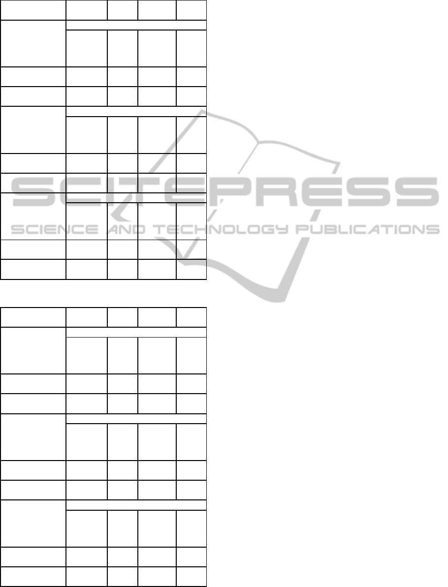
Table 4: Leukemia dataset.

Precision Recall F-

Measure

ROC

Area

Relief

0.933 0.894 0.913 0.865

Inf Gain 0.913 0.894 0.903 0.871

Correlation 0.933 0.894 0.913 0.865

Mean Aggreg

0.951 0.83 0.886 0.866

GA(Kendall) 0.955 0.894 0.923 0.899

GA(Spearman) 0.952 0.851 0.899 0.878

SVM

Relief

0.972 0.972 0.972 0.969

Inf Gain 0.93 0.931 0.93 0.919

Correlation 0.958 0.958 0.958 0.949

Mean Aggreg

0.972 0.972 0.972 0.969

GA(Kendall) 0.986 0.986 0.986 0.98

GA(Spearman) 0.972 0.972 0.972 0.969

KNN

Relief

0.944 0.944 0.944 0.936

Inf Gain 0.92 0.917 0.917 0.92

Correlation 0.93 0.931 0.93 0.911

Mean Aggreg

0.973 0.972 0.972 0.951

GA(Kendall) 0.973 0.972 0.972 0.951

GA(Spearman) 0.958 0.958 0.958 0.938

Table 5: Central Nervous System dataset.

Precision Recall F-

Measure

ROC

Area

Relief

0.600 0.538 0.568 0.399

Inf Gain 0.674 0.744 0.707 0.535

Correlation 0.676 0.641 0.658 0.512

Mean Aggreg

0.73 0.692 0.711 0.589

GA(Kendall) 0.795 0.795 0.795 0.74

GA(Spearman) 0.821 0.821 0.821 0.749

SVM

Relief

0.632 0.615 0.623 0.474

Inf Gain 0.737 0.718 0.727 0.621

Correlation 0.700 0.718 0.709 0.573

Mean Aggreg

0.825 0.846 0.835 0.756

GA(Kendall) 0.805 0.846 0.825 0.733

GA(Spearman) 0.875 0.897 0.886 0.83

KNN

Relief

0.659 0.692 0.675 0.513

Inf Gain 0.727 0.615 0.667 0.593

Correlation 0.677 0.538 0.600 0.531

Mean Aggreg

0.837 0.923 0.878 0.795

GA(Kendall) 0.787 0.949 0.86 0.736

GA(Spearman) 0.841 0.949 0.892 0.808

dataset, GA with Spearman distance function gives

very good results and outperforms GA with Kendall

distance and mean aggregation for the three classiﬁ-

cation algorithms. Performance results of this algo-

rithm are especially excellent when using KNN clas-

siﬁer. GA with Kendall distance outperforms mean

aggregation for DT, but they have competitive results

for SVM and KNN classiﬁers. The performance im-

provement with all aggregation techniques comparing

to individual feature selection methods is very notice-

able for this dataset.

To summarize, we can notice that the achieved re-

sults show that the fusion performance is either supe-

rior to or at least as good as individual ﬁlter methods.

This conﬁrms the theoretical assumption that rank ag-

gregation provides the means of combining informa-

tion from individual ﬁltering methods and at the same

time overcome their weakness.

6 CONCLUSIONS

In this paper we present an overview of some of the

available ranking feature selection approaches. To get

the best results of all available alternatives, we com-

bine their results using rank aggregation. We demon-

strate that our rank aggregation algorithm can be used

to efﬁciently select important features based on differ-

ent ﬁltering criteria. We effectively combine the ranks

of a set of ﬁlter methods via a weighted aggregation

that optimizes a distance criterion using genetic al-

gorithm. We illustrate our procedure using four real

datasets from biological and ﬁnancial ﬁelds.

REFERENCES

Borda, J. C. D. (1781). Memoire sur les elections au scrutin.

Bouckaert, R. R., Frank, E., Hall, M., Kirkby, R., Reute-

mann, P., Seewald, A., and Scuse, D. (2009). Weka

manual (3.7.1).

Carterette, B. (2009). On rank correlation and the distance

between rankings. In Proceedings of the 32nd inter-

national ACM SIGIR conference on Research and de-

velopment in information retrieval, SIGIR ’09, pages

436–443, New York, NY, USA. ACM.

Caruana, R., Sa, V. R. D., Guyon, I., and Elisseeff, A.

(2003). Beneﬁtting from the variables that variable se-

lection discards. jmlr, 3: 12451264 (this issue. pages

200–3.

Clegg, J., Dawson, J. F., Porter, S. J., and Barley, M. H.

(2009). A Genetic Algorithm for Solving Combina-

torial Problems and the Effects of Experimental Error

- Applied to Optimizing Catalytic Materials. QSAR

& Combinatorial Science, 28(9):1010–1020.

KDIR2013-InternationalConferenceonKnowledgeDiscoveryandInformationRetrieval

DeConde, R., Hawley, S., Falcon, S., Clegg, N., Knudsen,

B., and Etzioni, R. (2006). Combining results of mi-

croarray experiments: A rank aggregation approach.

Statistical Applications in Genetics Molecular Biol-

ogy, 5(1):1–17.

Dinu, L. P. and Manea, F. (2006). An efﬁcient approach for

the rank aggregation problem. Theor. Comput. Sci.,

359(1):455–461.

Dwork, C., Kumar, R., Naor, M., and Sivakumar, D. (2001).

Rank aggregation methods for the web. pages 613–

622.

Ferri, C., Hern´andez-Orallo, J., and Modroiu, R. (2009).

An experimental comparison of performance mea-

sures for classiﬁcation. Pattern Recognition Letters,

30(1):27–38.

Golub, T. R., Slonim, D.K., Tamayo, P., Huard, C., Gaasen-

beek, M., Mesirov, J. P., Coller, H., Loh, M. L., Down-

ing, J. R., Caligiuri, M. A., and Bloomﬁeld, C. D.

(1999). Molecular classiﬁcation of cancer: class dis-

covery and class prediction by gene expression moni-

toring. Science, 286:531–537.

Gotshall, S. and Rylander, B. Optimal population size and

the genetic algorithm.

Guyon, I. and Elisseff, A. (2003). An introduction to vari-

able and feature selection. Journal of Machine Learn-

ing Research, 3:1157–1182.

Hall, M. A. (2000). Correlation-based feature selection for

discrete and numeric class machine learning. In Pro-

ceedings of the Seventeenth International Conference

on Machine Learning, pages 359–366. Morgan Kauf-

mann.

Hastie, T., Tibshirani, R., and Friedman, J. (2001). The

Elements of Statistical Learning. Springer series in

statistics. Springer New York Inc.

Holland, J. H. (1992). Adaptation in natural and artiﬁcial

systems. MIT Press, Cambridge, MA, USA.

Kira, K. and Rendell, L. (1992). A practical approach to

feature selection. In Sleeman, D. and Edwards, P., ed-

itors, International Conference on Machine Learning,

pages 368–377.

Kohavi, R. and John, G. H. (1997). Wrappers for feature

subset selection. Artiﬁcial Intelligence, 97:273–324.

Kumar, R. and Vassilvitskii, S. (2010). Generalized dis-

tances between rankings. In Proceedings of the 19th

international conference on World wide web, WWW

’10, pages 571–580, New York, NY, USA. ACM.

Okun, O. (2011). Feature Selection and Ensemble Methods

for Bioinformatics: Algorithmic Classiﬁcation and

Implementations.

Pomeroy, S. L., Tamayo, P., Gaasenbeek, M., Sturla, L. M.,

Angelo, M., McLaughlin, M. E., Kim, J. Y. H., Goum-

nerova, L. C., Black, P. M., Lau, C., Allen, J. C.,

Zagzag, D., Olson, J. M., Curran, T., Wetmore, C.,

Biegel, J. A., Poggio, T., Mukherjee, S., Rifkin, R.,

Califano, A., Stolovitzky, G., Louis, D. N., Mesirov,

J. P., Lander, E. S., and Golub, T. R. (2002). Prediction

of central nervous system embryonal tumour outcome

based on gene expression. Nature, 415(6870):436–

442.

Quinlan, J. R. (1993). C4.5: programs for machine learn-

ing. Morgan Kaufmann Publishers Inc.

Vafaie, H. and Imam, I. (1994). Feature Selection Meth-

ods: Genetic Algorithms vs. Greedy-like Search.

Manuscript.

Weston, J., Elisseeff, A., Schlkopf, B., and Kaelbling, P.

(2003). Use of the zero-norm with linear models and

kernel methods. Journal of Machine Learning Re-

search, 3:1439–1461.

Young, H. P. (1990). Condorcet’s theory of voting. Math-

matiques et Sciences Humaines, 111:45–59.

Young, H. P. and Levenglick, A. (1978”,). A consistent ex-

tension of Condorcet’s election principle. SIAM Jour-

nal on Applied Mathematics, 35(2):285–300.

FeatureSelectionbyRankAggregationandGeneticAlgorithms