Average Speed Estimation for Road Networks based on GPS Raw

Trajectories

Ivanildo Barbosa

1,2

, Marco Antonio Casanova

Chiara Renso

and José Antônio Fernandes de Macedo

Military Institute of Engineering, Rio de Janeiro, Brazil

Department of Informatics, Pontifical Catholic University, Rio de Janeiro, Brazil

KDDLAB, ISTI-CNR, Pisa, Italy

Department of Computer Science, Federal University of Ceará, Fortaleza, Brazil

Keywords: Geospatial Data Mining, Smart Routing, Traffic Modeling.

Abstract: For applications involving displacements around cities, planners cannot count on moving at the legal speed

limits. Indeed, the amount of circulating vehicles decreases the average speed and consequently increases

the estimated time for daily trips. On the other hand, the number of available trajectories generated by GPS

devices is growing. This paper presents a methodology to compute statistics about a road network based on

GPS-tracked points, generated by vehicles moving around a city. The proposed methodology allows

selecting the most representative data to describe how speeds are distributed along the days of week as well

as along the time of the day. The results obtained may be used as an alternative to the shortest-path routing

criterion for route planning.

1 INTRODUCTION

Large cities face the problem of balancing the traffic

demand and the existing road network capacity.

Whenever the traffic demand exceeds the network

capacity, queuing is expected, average speeds

decrease and traffic congestions occur, implying

longer trips, which is a relevant aspect to consider.

Traffic conditions are indeed relevant for route

planning to optimize the available resources. By

choosing the shortest path, we assume that the

speeds are the same at every road of a network.

However, different traffic demands, which are

typically time-dependent, lead to fluctuations on the

average speed value. It means that the shortest path

is not always the fastest option when planning a

route.

By using both the average speed and the length

of the roads, travel time may be estimated, which is

highly relevant for planning applications with

predefined deadlines for displacements. These

values may also be used as benchmarks for

monitoring vehicles: low speeds may indicate that

replanning is required or that some kind of

emergency has to be mitigated (Albuquerque et al.,

2012).

The speeds may be computed from consecutive

locations captured by GPS receptors available as

independent devices or embedded in mobile phones.

Data from mobile phones must be carefully filtered

because the devices may be stopped inside the

buildings, stopped or moving slowly at sidewalks

instead of considering only the people inside the

vehicles. Moreover, inside a bus we could consider a

set of devices within a single vehicle supposed to

move slower and to stop more frequently. The

second alternative, GPS devices facilitate, in

principle, collecting data about any road along the

network at a low cost. Furthermore, a GPS attached

to a moving vehicle makes it possible to track the

trajectory of the vehicle. The main disadvantage in

this approach is the sample size required to model

real traffic conditions, which may be addressed by

increasing both the tracking ratio (spatially or

temporally) and the number of vehicles enabled with

GPS receptors capable of providing data.

This paper proposes a methodology to enrich a

road network database with statistics about the

actual speeds, based on an analysis of raw

trajectories relative to vehicles moving around a

city. The computed statistics consists of the average

speed, the standard deviation and the sample size

490

Barbosa I., Antonio Casanova M., Renso C. and Antônio Fernandes de Macedo J..

Average Speed Estimation for Road Networks based on GPS Raw Trajectories.

DOI: 10.5220/0004450904900497

In Proceedings of the 15th International Conference on Enterprise Information Systems (ICEIS-2013), pages 490-497

ISBN: 978-989-8565-59-4

 2013 SCITEPRESS (Science and Technology Publications, Lda.)

used in computations assigned to individual

instances of roads and refers to predefined time

intervals. These average speed values are useful to

estimate the travel time for a vehicle along candidate

routes to assess how fast they are. The fluctuations

of speed values along the time are also considered.

To achieve the proposed objective, the

methodology performs three main steps: (1) map-

matching (2) temporal partition of GPS points and

(3) statistics computation and road segment

enrichment.

The purpose of the first step on map-matching is

to correctly match GPS points and road geometries.

This is indeed a problem due to: (1) inaccuracies in

the road geometries and the lack of information

about the road widths; (2) inaccuracies of GPS data.

When combined, these two sources of problems

imply that the GPS tracked points may not exactly

fit road geometries. Some points must not be

considered because they were tracked out of the road

(such as at parking lots, at private or at unmapped

ways). We introduce the direction analysis to

improve the results returned by this step.

The second step is the temporal partition of GPS

points. The partition criterion must model speed

fluctuations to compute consistent statistics based on

a representative amount of data. The larger the

sample is, the more representative the results will be.

We then discuss how to balance between these two

aspects.

The last step refers to the computation of

statistics of the temporally partitioned GPS points

and adding these statistics to the original road

network data.

The paper is organized as follows. Section 2

describes the problem statement and the model used

to address the proposed scenario. Section 3 explains

the methodology adopted to extract the average

speed information from the raw data. Session 4

reports on the experimental results of an application.

Session 5 presents related works. Finally, Section 6

contains the conclusions and final remarks.

2 PROBLEM STATEMENT

The approach presented in this paper assumes the

following scenario. A generic moving vehicle is

tracked using a GPS device. The vehicle leaves a

location called the origin where the trip starts and

moves through a set of roads towards another

location called the destination where the trip ends.

The path from the origin to the destination is decided

by a plan. The roads in the path are represented by

polylines and the plan is supposed to consider that

every consecutive road is connected. The plan may

choose the route whose total length is minimal or

consider the route with minimum travel time, based

on the average speed the vehicles may achieve on

each route.

The input data, generated by the GPS devices, is

represented as a tuple

P = <i, p, t, v, s>

where:

 i is the (anonymous) user reference

 p is the point geometry, in WGS-84 geodetic

coordinates

 t is the timestamp, with time zone, when the point

was tracked

 v is the instantaneous speed value

 s indicates the tracking status during a single trip: 0

for start point, 2 for end point and 1 otherwise (no

data is recorded when the vehicle is turned off,

even if it is parked along a road.

We assume that the instantaneous speed, location

and timestamp are simultaneously stored. Moreover,

we assume that the informed instantaneous speed is

accurate.

Each road segment is represented as a tuple

R = <w, l, n, o>

where:

 w is a unique identifier of the road segment

 l is the road segment geometry

 n is the name of the road

 o is the allowed traffic directions (one-way or two-

way road).

Therefore, a road segment corresponds to a

geometric element used to represent an entire road

or a part of a road (different directions or portions

between relevant crossings).

The problem we propose to solve is: given a

dataset containing the GPS tracks of moving

vehicles and a dataset containing road network data,

we want to compute, for each road, the time

dependent average speed, standard deviation and the

sample size computed. This additional information is

then attached to the original road data thereby

creating an enriched road segment.

An enriched road segment is a tuple

S = <w, l, n, o, k, h, a, d, c

The first four elements correspond to the

respective road segment R

= <w, l, n, o> enriched

with:

 k is the day of week (‘0’ for Sunday up to ‘6’,

AverageSpeedEstimationforRoadNetworksbasedonGPSRawTrajectories

491

Saturday)

 h is the time interval (e.g., from ‘0’ to ‘23’ for 1-

hour time intervals along the day)

 a is the average speed

 d is the standard deviation

 c is the number of points considered.

3 DATA PROCESSING

Figure 1 illustrates the process of building the

enriched road segments from the two raw datasets

containing GPS tracks and road geometries. The

first phase performs the map matching process. The

second phase performs the data analysis on the road

segments to both identify and eliminate the

mismatches returned by the previous phase by

analyzing the direction that vehicles move along.

The third step performs a temporal classification of

the GPS map-matched points into predefined

temporal intervals like the hour of the day and the

day of the week. Finally statistics are computed and

the road segments are enriched with them. In the

next sections we illustrate the details of each step.

3.1 Map Matching

Recall that the points were tracked along the

vehicles’ trajectories. Hence, since vehicles move

along roads, we may assume that they are associated

with a road segment, represented as a linear

geometry.

This is a problem known in the literature as map

matching, where methods to assign GPS points to a

road segment are proposed. Modern techniques of

map matching have been developed. See

Brakatsoulas et al (2005) for some algorithms

proposed to deal the map matching process.

However, in this context, off-roads points must

not be considered due to the bias they may insert in

the statistics. It is necessary to select only the points

supposed to be moving along the instances of the

road database available and discard the off-road

points. The solution we adopted to address this issue

is to define a buffer zone around each road segment

and to associate each point to a unique road

segment, or to discard the point. Not only off-road

movements are discarded: this step removes low-

accuracy points tracked.

The main related issue is to define how wide the

buffer zone is: low width values potentially imply

discarding useful points to improve the statistics;

higher values imply the selection of points out of the

range of the road (such as vehicles on another near

road or stopped at the road shoulders). The width

value for these buffer zones should be compatible

with the respective real road width, when available.

Indeed, due to the lack of data about road widths,

during the experiments, we considered 3 meters, 5

meters and 8 meters wide buffer zones.

When the buffer zones overlap, the risk of a

point-road mismatching increases. Aiming at

minimizing the mismatches in contexts where an

individual vehicle and the traffic flow in opposite

directions, we propose to analyze the direction of

movement, as presented at the next section.

3.2 Direction Analysis

Directions are computed as the azimuth of the line

defined by an ordered pair of points O

= <P

, P

i+1

tracked by the same vehicle at the same trajectory

and ordered by their timestamp. By pairing

consecutive points, it becomes feasible to indicate

the direction of the movement of an individual

vehicle. From now on we refer to these pairs of

points as oriented points because of the implicit

orientation quantified by the azimuth.

As modelled in Section 2, each road segment has

information about the traffic direction: one-way or

two-way roads.

The direction analysis step considers three cases:

a) One-way Road and Single Geometry: all

Figure 1: Proposed process steps to enrich data about roads with statistics about speed.

Data Analysis Map Matching

Road

geometries

Raw GPS

oints

Buffer zones

definition

Filtering by

buffer zones

Direction

Analysis

Temporal

classification

Statistics

Computation

One-way?

Two-ways

traffic

Road Geometries

with statistics

ICEIS2013-15thInternationalConferenceonEnterpriseInformationSystems

492

vehicles move along (or nearly along) the road

bearing, indicated as Az

, and the distribution of

those values reflects the road geometry.

b) Two-way Road and Single Geometry: the

bearing values are grouped close to the road

bearing indicated as Az

and to Az

± 180°.

c) Two-way Road and Distinct Geometry: the

bearing values are grouped close to the road

bearing Az

. However, due to the proximity of

the road geometries, some values close to Az

180° may occur, probably referred to another

buffer zone.

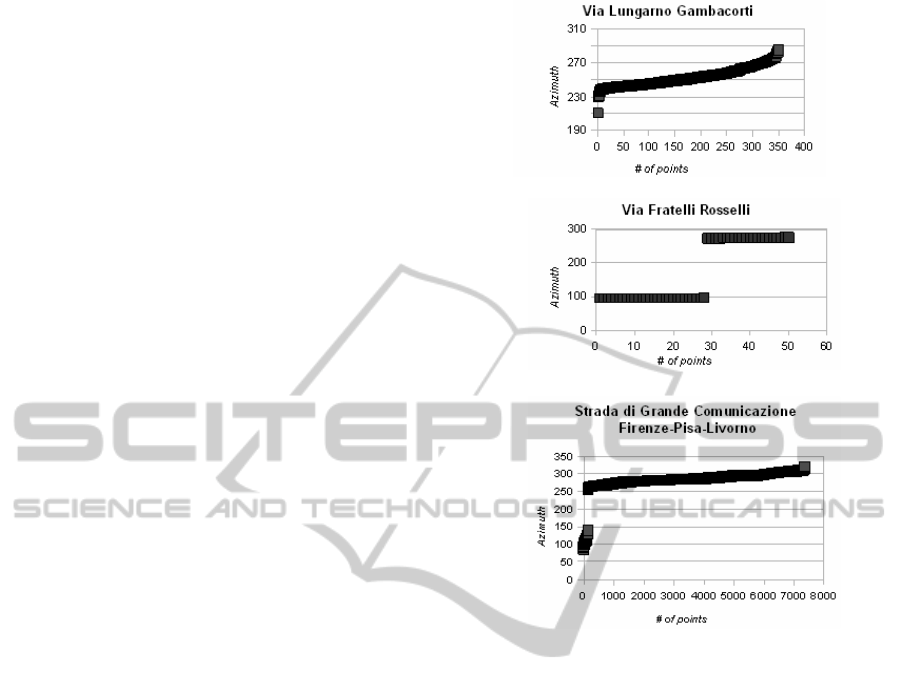
The Figure 2a illustrates the distribution of the

azimuth values along Via Lungarno Gambacorti, an

example of the first case. The continuous

distribution of values suggests that every vehicle

following the same direction even in curvilineous

roads.

The Figure 2b illustrates the distribution of the

azimuth values along Via Fratelli Rosselli, a two-

way road represented as a single line. It is possible

to identify two groups of values near Az

and the

opposite direction, Az

+ 180º, as consequence of

two-way traffic. It is also possible to identify the

ratio of vehicles flowing in each direction. By

computing meaningful statistics for the respective

road we must distinguish the traffic flow on opposite

directions.

The Strada di Grande Comunicazione Firenze-

Pisa-Livorno is an example of two-way road with

distinct geometries, i.e., each direction is represented

individually. The geometries are usually adjacent

and this therefore leads the risk of point-road

mismatch. The distribution illustrated at the Figure

2c refers to the points tracked along one direction of

the Strada. We can identify two groups, despite the

fact that the geometry is supposed represent one

single direction: a small number of outliers is then

detected and, by discarding them, statistics may be

improved.

As the directions are supposed to be opposite, the

method proposes to group the oriented points by

their azimuths: the first group, closer to the average

value (A), and the second one (with outliers), closer

to A plus 180°, considering the cyclic nature of

bearing as an angular measure. Azimuth values

closer to A were considered for statistics

computations.

However, this rule does not work when two-

ways roads are represented by a single geometry

(Figure 2b) because we do not know the traffic

distribution ratio between both directions. A

possibility to solve this problem could be to apply

(a)

(b)

(c)

Figure 2: Distribution of azimuth values for oriented

points.

clustering techniques to group the azimuth values

into two groups, which would permit to identify the

traffic in each direction. This feature has not yet

been implemented in the system.

We call attention to the low ratio of oriented

points O

considered, as a consequence of taking into

account only the pairs tracked in the buffer zone and

along the same road R

. On the other hand, when we

assume that P

and P

i+1

may be assigned to different

roads, the number of oriented points O

increases.

For longer tracking rates, it would be necessary to

infer the path between consecutive points located on

different roads.

Another issue to handle is the overlapping of

buffer zones. If P

i+1

is located at the intersection of

buffer zones related to different roads, R

and R

, a

simple query may assign both roads to the point. The

preferred solution considers the buffer zone that

contains both points.

Since we aim at eliminating sources of

uncertainty, we adopted the approach that takes into

account only the pairs tracked in the buffer zone and

AverageSpeedEstimationforRoadNetworksbasedonGPSRawTrajectories

493

along the same road R

even if it reduces the number

of points considered for the computation.

3.3 Temporal Classification

One specific contribution of this work is to provide

time-dependent enriched road segments. This means

that the average speed associated with each road

segment is split into temporal intervals, which

represent the average speed in during that particular

time interval. This information improves the

planning of a route from an origin and a destination

by considering the traffic dynamics along the day

(and along the week). Therefore, to provide this

information, we need to classify the speeds in short

time intervals, either predefined or established based

on the amount of tracked vehicles.

3.4 Statistics Computation

At this phase, the original data are organized as

oriented points associated with the road segments

and classified according to the day of week and the

hour they were tracked. Arithmetic average,

standard deviation and the number of points

considered for the filtered data are then computed.

The average indicates the main reference for the

expected speed for the road; the standard deviation

indicates how the observed values may vary (high

values for the standard deviation may also indicate

some anomaly on the traffic). The number of points

considered for the statistics may be used to indicate

how reliable the computed values are or to support

the estimation of confidence intervals. The results

are then stored as new attributes of the respective

road segment, following the enriched road segment

model introduced in Section 2.

4 EXPERIMENTAL RESULTS

4.1 Application using Real Datasets

The datasets considered for the experiments are: (1)

points tracked by GPS receptors installed at 8,575

vehicles, in the period between May 1st and May

31st, 2011; (2) geometries of the roads in the region

analyzed, extracted from the Open Street Map

repository.

The points tracked in this region were ordered by

the users' identification and by timestamp, so as to

analyze the behavior of each vehicle.

The original dataset containing the raw GPS

points contained 163,278,486 records. This number

reduces to 1,020,909 when we consider the

predefined geographical extents. After the pairing

process, there were 783,622 oriented pairs of points.

The road network comprises 1,555 records, among

which only 1,057 are named (the unnamed roads are

bicycle or pedestrian ways). Among these, 309 are

one-way roads.

The results achieved after filtering the points by

the buffer zones are illustrated in Table 1. The first

column contains the values of the widths we

considered to compose the statistics. The second

column indicates the number of raw points within

the buffer zone, as well as the proportion when

compared to the number of the available points.

Analogously, the third column indicates how many

oriented points are within the buffer zone, as well as

the proportion when compared to the number of the

available oriented points. The fourth column refers

to the roads whose statistics could be computed

based on the existing points and the proportion

considering the existing roads on the network.

Table 1: Statistics for processing results.

Width

(m)

Raw Points

Oriented Points

Roads with

enriched data

352,221

34.5%

23,997

3.06%

249

23.6%

557,555

54,6%

55,574

7.09%

329

31.1%

792,639

77.6%

97,871

12.5%

415

39.3%

As expected, the number of points increases when

the buffer zone width increases. However, the ratio

is not constant: it is higher for lower widths.

Table 2 introduces further statistics. The first and

the second columns correspond, respectively, to the

first and third columns of Table 1. The values on the

third column represent the number of one-way roads

enriched with speed statistics: the proportion refers

to the number of one-way roads at the roads dataset.

The fourth column presents the number of oriented

points erroneously assigned to roads and the

respective proportion related to the number of

oriented points. These points were discarded for

statistics computations.

By considering the temporal classification, for

these tests, the points were divided in 1-hour

intervals based on their respective timestamps. To

analyze the fluctuation along the week, they were

also classified according to the day-of-week. Recall

that these data were partitioned by the days of week

and refer to 4 weeks. This means, for example, that

ICEIS2013-15thInternationalConferenceonEnterpriseInformationSystems

494

the four Mondays are collapsed into one day

representing the typical Monday in the observed

period.

Table 2: Additional statistics for processing results.

Width

(m)

Oriented

Points

One-way

Roads

Mismatches

Point - Road

23,997

3.06%

28.5%

205

0,85%

55,574

7.09%

113

36.6%

602

1,08%

97,871

12.5%

143

46.3%

2263

2,31%

After performing the distribution of average speeds

along the week, further to the main objective – to

use average speeds to estimate travel time, atypical

behaviors can be detected. An individual analysis is

necessary to assess whether the observed values

affects the meaning of the computed statistics.

For some roads, no points were tracked along

some time interval or were selected after the filtering

processes we described. Therefore, no statistics were

computed. For missing values, we suggest some

strategies: (1) assign the nominal speed for the road

– there is no traffic flow enough to justify lower

values for speed; (2) interpolate the values from the

nearest intervals – for isolated lacks of values; or (3)

assign zero as the speed value – travel time is too

high to be considered due to the uncertainty in speed

values.

4.2 Travel Time Prediction

An example of application of the enriched road

segments is the travel time estimation based on the

pre-computed average speeds. A well-known

location has been adopted as the origin of a planned

trip, while the destination is a given address chosen

in the urban area across the city.

Three routes were proposed by the Google Maps

service, represented by the names of the roads and

the respective lengths (Figure 3). By considering the

travel time the sum of the ratios length / average

speed for every road, we compute the total travel

time in these three options. The computations are

summarized in Table 3 and the values refer to the

interval 4 – 5 p.m. for Tuesdays.

Table 3: Travel times based on pre-computed average

speeds.

Route

Total

length (m)

Travel time for buffer width

3m 5m 8m

Google

Maps

1 3402 13’ 48” 13’ 5” 13’ 48” 8’

2 3308 15’ 13” 14’ 32” 15’ 11” 11’

3 4015 15’ 35” 14’ 44” 15’ 14” 11’

By comparing routes #1 and #2, we highlight

that the shortest path is not the faster. Although

route #3 is the longest one, the average speed along

it is the highest, when compared to the other routes.

Moreover, route #3 could be considered because the

travel time along it is not much longer than that

along route #2. The results provided by the Google

service suggest faster displacements however we get

the same conclusions comparing the routes.

Therefore, planners may also consider the average

speed to support decision making.

By repeating the procedures for route #1 on

Thursdays in the interval of 3 – 4 p.m., the computed

travel time is 15’ 32”, approximately 2’ slower than

the result at the first time interval. For longer trips,

these delays may accumulate and achieve critical

values. In cities where traffic is heavier, fluctuations

for average speed values tend to be more noticeable.

(a) (b)………………………………………………………(c)

Figure 3: Options of routes for movement planning.

AverageSpeedEstimationforRoadNetworksbasedonGPSRawTrajectories

495

5 RELATED WORK

To provide reliable resources for planning involving

moving objects, methodologies were developed to

predict the movement dynamics in uncertain

contexts. In fact, by moving along road networks

(specially in urban zones), mobile users usually have

no idea about how many cars are moving with them,

where they come from and where they are going.

However, these users are free to choose another

route (unless it is mandatory, such as on the buses)

to try to find the shortest time solution.

Raw locations tracked by GPS receptors have

been used for controlled applications such as buses

and trucks private fleets. Masiero et al. (2011)

present a methodology based on Support Vector

Regression (SVR) to predict the travel time for

delivery trucks based on previous trajectories.

Sinn et al. (2012) describe another application

for time travel prediction from GPS points. In

addition, they present a method to automatically

extract bus routes, stops and schedules. In all these

cases, the analysis considered fixed trajectories

(stops and moves) and controlled speeds. Pang et al

(2011) proposed another methodology for time

travel prediction based in GPS data on buses.

However they use smart phones to gather data for

the analysis. In addition, they present a method to

automatically extract the bus routes, the stops and

the schedules. In all of these three cases, the analysis

considered fixed trajectories (stops and moves) and

controlled speeds. Hence, the tracked data is not

representative to model the global average speed for

a road network.

The method presented in Min and Wynter (2011)

is based on spatial-correlation matrices and average

speeds obtained from historical data of some

categories of roads and provides predictions of speed

and volume over 5-min intervals for up to 1 h in

advance.

The analysis presented by Yuan et al. (2011) is

based on GPS data relative to three months of GPS

trajectories collected from 33,000 taxis in Beijing to

detect anomalies on traffic behavior. Although taxis

trajectories are supposed to be more flexible, they

are influenced by the existence of either permanent

or temporary points of interest such as touristic

places, airports, hotels or convention centers.

On the other hand, in Biagioni et al. (2011), the

taxis drivers' intelligence in choosing faster routes is

modeled by analyzing the trajectories they usually

take. In this case, the traversing frequencies along

the road network are considered instead of speeds.

Therefore, this method ranks the streets by the

drivers’ preferences (as consequence of their

previous experiences).

Letchner et al. (2006) present a method that

considers the previous individual history (i. e., the

user’s preferences) to indicate routes for general

users (instead of taxi drivers).

Our contribution is the generation of more

representative statistics based on the actual behavior

of non-specific groups of drivers or categories of

roads.

6 CONCLUSIONS

We proposed a methodology to enrich a road

network database with statistics about the actual

speeds, based on the analysis of raw trajectories

tracked by usual vehicles during one month. These

results reflect how traffic flow behaves along the

days of the week and the hours of each day of week

– although the methodology allows different time

intervals. Moreover, they will support movement

planning by proposing routes based on the estimated

travel time instead of the travel length.

The method is based on three steps: (1) map-

matching (2) temporal partition of GPS points and

(3) statistics computation and road segment

enrichment. Because of inaccuracies on GPS

positioning and off-roads points, we limited the

analysis to the points tracked near the roads – the

buffer zones, which width must be compatible to the

real width of the respective road.

The combined analysis of tables 1 and 2 shows

that, by enlarging the buffer zones, the gain in the

number of oriented points is limited. Furthermore,

among these points, the ratio of outliers increases

fast. The direction analysis detected outliers, even by

reducing the size of the sample of GPS points.

Despite the mismatches, the number of one-way

roads with enriched data increases because most of

the additional mismatches occurred just in a few

roads.

Atypical behavior can also be detected. In these

cases, some observations must be discarded to keep

the statistics meaningful.

We emphasize that many of the computed

statistics considered too few points for each time

interval. By considering 3-meter wide buffer zones,

82% of the records are computed based on less than

10 points. The ratio for records, such as these, in the

5- and 8-meter wide buffer zones respectively are,

79% and 76% (we do not consider this a

representative gain). To increase this percentage, the

methodology must be improved to consider more

ICEIS2013-15thInternationalConferenceonEnterpriseInformationSystems

496

oriented points by adopting pairs of consecutive

points inside the buffer zones created near different

instances of road. However, some additional

discussion is necessary to filter inconsistencies and

ambiguities mentioned at the section 3.B.

In future research, the analysis used by Biagioni

et al. (2011) based on the frequencies may be

combined with the spatio-temporal distribution of

tracked points. Another approach to handle this issue

is to apply the algorithm presented by Lou et al

(2009) to propose candidate paths along low-

sampling-rate GPS trajectories.

We may also consider the adaptive fastest path

algorithm presented by Gonzalez et al. (2007) that is

based on the leverage of the hierarchy of roads, on

limiting the route search strategy to edges and path

segments that are actually frequently traveled in the

data, and on the road widths.

Another future improvement to be implemented

is the adaptive temporal classification by adopting

finer intervals (1-hour or 15 minutes) for larger

samples and wider intervals for smaller samples (the

entire day or morning-afternoon-evening). The lack

of data for these streets means that users prefer not

to use them in their trips due to the low speed or bad

conservation.

As for future work, the results we achieved with

GPS raw trajectories may be combined with data

from other sources (such as loop detectors and

mobile phones) to obtain statistics based on larger

samples. Moreover, the functionalities to handle the

cases when two-ways roads are represented by a

single geometry, as indicated at the Section 3.2.

ACKNOWLEDGEMENTS

This work was mainly supported by EU project FP7-

PEOPLE SEEK (No. 295179).

REFERENCES

Albuquerque, F. C., Barbosa, I., Casanova, M. A., de

Carvalho, M. T. M., de Macedo, J. A. F., 2012. Pro-

active monitoring of moving objects. In ICEIS’12,

14th International Conference on Enterprise

Information Systems (ICEIS).

Brakatsoulas, S., Pfoser, D., Salas, R., Wenk, C. 2005. On

map-matching vehicle tracking data. In VLDB’05, 31st

international conference on Very large data bases.

Biagioni, J.; Gerlich, T.; Merrifield, T.; Eriksson, J. 2011.

EasyTracker: Automatic Transit Tracking , Mapping ,

and Arrival Time Prediction Using Smartphones. In

9th ACM Conference on Embedded Networked Sensor

Systems, Pages 68-81.

Lou, Y., Zhang, C., Zheng, C., Xie, X. Wang, W., Huang,

Y. 2009. Map-matching for low-sampling-rate GPS

trajectories. In 17th ACM SIGSPATIAL International

Conference on Advances in Geographic Information

Systems.

Masiero, L., Casanova, M.A., Carvalho, M.T.M. 2011.

Travel Time Prediction using Machine Learning. In

IWCTS’11, 4th ACM SIGSPATIAL International

Workshop on Computational Transportation Science.

Min, W., and Wynter, L. 2011.Real-time road traffic

prediction with spatio-temporal correlations. In:

Transportation Research Part C: Emerging

Technologies 19.4: 606-616.

Pang, L. X., Chawla, S. Liu, W., Zheng, Y. 2011. On

Mining Anomalous Patterns in Road Traffic Streams.

In 7th International Conference on Advanced Data

Mining and Applications.

Sinn, M.; Yoon J. W.; Calabrese , F. 2012. Predicting

arrival times of buses using real-time GPS

measurements, In 15th IEEE Intelligent

Transportation Systems Conference.

Yuan, J.; Zheng, Y.; Xie, X.; Sun, G. 2011. T-Drive:

Enhancing Driving Directions with Taxi Drivers'

Intelligence, In IEEE Transactions on Knowledge and

Data Engineering, vol. PP, no.99.

AverageSpeedEstimationforRoadNetworksbasedonGPSRawTrajectories

497