
Adding Recommendations to OLAP Reporting Tool
Natalija Kozmina
Faculty of Computing, University of Latvia, Raina blvd. 19, Riga, Latvia
Keywords: OLAP Personalization, Report Recommendations, Data Warehouse Reporting.
Abstract: In this paper an example of applying the recommendation component of OLAP reporting tool developed
and put to operation at the University is presented. To construct report recommendations in the above-
mentioned tool content-based methods are employed. Analyzing user activity and taking advantage of data
about user preferences for data warehouse schema elements existing reports that potentially may be
interesting to the user are distinguished and recommended. The approach for recommending reports is
composed of two methods – cold-start and hot-start. The cold-start method is employed, if a user is either
new to the system or classified as passive, while the hot-start method is applied for active system users.
Both methods are implemented in OLAP reporting tool. The recommendation component of the OLAP
reporting tool is presented, and different recommendation modes are described.
1 INTRODUCTION
OLAP applications are built to perform analytical
tasks within a large amount of multidimensional
data. During working sessions with OLAP
applications the working patterns can vary. Due to
the large volumes of data the typical OLAP queries
performed via OLAP operations by users may return
too much information that sometimes makes data
exploration burdening or time-consuming. If there
are too many constraints, the result set can be empty.
In other cases, when the user explores previously
unknown data, OLAP query result may differ from
user’s expectations. Therefore, a user is rather
limited in expressing his/her likes and dislikes to get
the results that are more satisfying.
The experience in using standard applications for
producing and managing data warehouse reports (for
instance, Oracle Discoverer and MicroStrategy) at
the University as well as participation in scientific
projects and development of a new data warehouse
reporting tool (Solodovnikova, 2007) served as a
motivation for further studies in the field of OLAP
personalization, so that the users of the reporting
tool would not only create, modify and execute
reports on data warehouse schema but also acquire
some extra information such as recommendations on
what else to examine. Users of the reporting tool
may have different skill levels (e.g., expert, novice),
which is why reports’ recommendations based on
user preferences are more valuable for novice users
than for experts. The reporting tool is a part of the
data warehouse framework developed at the
University.
The research made in the field of personalization
in OLAP was summed up in our previous works
(Kozmina and Niedrite, 2011); (Kozmina and
Niedrite, 2010). In (Kozmina and Niedrite, 2011) we
have provided an evaluation in order to point out (i)
personalization options described in existing
approaches, and their applicability to OLAP schema
elements, acceptable aggregations, and OLAP
operations, (ii) the type of constraints (hard, soft or
other) used in each approach, and (iii) methods for
obtaining user preferences and collecting user
information. In (Kozmina and Niedrite, 2010) a new
method to describe interaction between user and
data warehouse was proposed, as well as a model to
formalize user preferences was presented. To
develop user preference metamodel, we considered
various user preference modeling scenarios, which
later were divided into two groups: (i) preferences
for the contents and structure of reports (OLAP
preferences), and (ii) visual layout preferences. In its
turn, OLAP preferences are of two types: schema-
specific, i.e., preferences for structure elements (e.g.,
OLAP schema, dimensions, fact tables, etc.) in
particular reports, and report-specific, i.e.,
preferences for data restrictions in reports. We
continued our work by developing an approach for
169
Kozmina N..
Adding Recommendations to OLAP Reporting Tool.
DOI: 10.5220/0004439801690176
In Proceedings of the 15th International Conference on Enterprise Information Systems (ICEIS-2013), pages 169-176
ISBN: 978-989-8565-59-4
Copyright
c
2013 SCITEPRESS (Science and Technology Publications, Lda.)

generating recommendations of reports based on
schema-specific OLAP preferences of a user in
(Kozmina and Solodovnikova, 2011). In terms of
this approach, all necessary data about user
preferences is gathered implicitly (i.e., without
asking the user to provide any information directly)
from the query log. The main methods of the
approach are recalled concisely in Section 4 of this
paper. Different usage scenarios of the
recommendation component applied to real data
warehouse reports on learning process are presented
in the actual paper.
The rest of the paper is organized as follows: in
Section 2 an overview of the related work is given,
Section 3 shortly describes the reporting tool and
provides its technical details, in Section 4 user
interaction with the recommendation component of
the reporting tool is presented, and Section 5
concludes the paper.
2 RELATED WORK
There are methods in traditional databases that
process user likes/dislikes to put query
personalization into action (Koutrika and Ioannidis,
2004). However, in the field of data warehousing
similar ideas are reflected in the recent works of
various authors on data warehouse personalization.
The data warehouse personalization itself has
many different aspects. Data warehouse can be
personalized at schema level (Garrigós et al., 2009),
employing the data warehouse multidimensional
model, user model and rules for the data warehouse
personalization to let a data warehouse user work
with a personalized OLAP schema. Users may
express their preferences on OLAP queries
(Golfarelli and Rizzi, 2009). In this case, the
problem of performing time-consuming OLAP
operations to find the necessary data can be
significantly improved. The other method of
personalizing OLAP systems is to provide query
recommendations to data warehouse users. OLAP
recommendation techniques are proposed in
(Giacometti et al., 2009) and (Jerbi, 2009). In
(Giacometti et al., 2009) former sessions of the same
data warehouse user are being investigated. User
profiles that contain user preferences are taken into
consideration in (Jerbi, 2009), while generating
query recommendations. Other aspect of OLAP
personalization is visual representation of data. In
(Mansmann and Scholl, 2007) authors introduce
multiple layouts and visualization techniques that
may be used interactively for different analysis
tasks. As it was mentioned above, we performed a
review of these approaches which can be observed
in (Kozmina and Niedrite, 2011). The main purpose
of this research was to become aware of the existing
state-of-the-art approaches in the field of data
warehouse personalization and to determine a
possible way of categorizing and comparing them.
Also, it was important to understand, whether there
is a superior approach, and if not then which of the
approaches would be the most suitable for
introducing personalization into the data warehouse
reporting tool of the University. In our case the
emphasis is put on presence of the large set of users
with different experience and knowledge about data
warehousing with their preferences interpreted as
soft constraints stated rather implicitly than
explicitly, whereas the visualization of results would
play a secondary role. Such characteristics refer to
both approaches that include query
recommendations (Giacometti et al., 2009) and
(Jerbi, 2009). Our approach presented in (Kozmina
and Solodovnikova, 2011) is different from other
approaches involving query recommendations,
because it produces the recommendations of another
kind. To be more specific, we do not look for
likeliness in reports’ data nor semantic terms, but the
likeliness on the level of logical metadata (i.e.,
OLAP schema, its elements and aggregate
functions) is revealed. Later other researchers
conducted a comparative study of OLAP
personalization approaches (Aissi and Gouider,
2012) and analyzed data warehouse personalization
techniques according to such criteria as user
characteristics, user context, user behavior, user
requirements, and user preferences.
Methodologies most commonly used in
recommender systems (Vozalis and Margaritis,
2003) have also been considered. Recommender
systems operate with such entities as users and
items. A user of the recommender system expresses
his/her interest in a certain item by assigning a rating
(i.e., a numeric equivalent of user’s attitude towards
the item within a specific numerical scale). In
(Vozalis and Margaritis, 2003) an overview and
analysis of algorithms employed in recommender
systems is presented. One may distinct user-based,
item-based and hybrid algorithms. User-based and
item-based methods refer to collaborative filtering.
Hybrid methods combine principles of both user-
based and item-based ones.
In the field of data warehousing a survey of the
existing methods for computing data warehouse
ICEIS2013-15thInternationalConferenceonEnterpriseInformationSystems
170

query recommendations is proposed in (Marcel and
Negre, 2011). Authors of the survey singled out four
methods that convert a user’s query into another one
that is likely to have an added value for the user: (i)
methods exploiting a profile, (ii) methods based on
expectations, (iii) methods exploiting query logs,
and (iv) hybrid methods.
3 OLAP REPORTING TOOL
The architecture of the reporting tool is composed of
the server with a relational database to store data
warehouse data and metadata, data acquisition
procedures that manage the metadata of the data
warehouse schema and reports, and reporting tool
components which are located on the web-server to
define reports, display reports and provide
recommendations on similar reports.
For the implementation of the reporting tool an
Oracle database management system was used. Data
acquisition procedures were implemented by means
of PL/SQL procedures. The Tomcat web server was
employed to allocate all the components of the
reporting tool. The components that define and
display reports as well as generate report
recommendations are designed as Java server
applets, which generate HTML code that can be
used in web browsers without any extra software
installation. For the graphical representation of the
reports an open source report engine called
JasperReports was taken.
All operation of the OLAP reporting tool is
based on metadata that consists of five
interconnected layers: logical, physical, semantic,
reporting, and OLAP preferences metadata. Logical
metadata is used to describe data warehouse
schemas. Physical metadata describes storage of a
data warehouse in a relational database. Semantic
metadata describes data stored in a data warehouse
and data warehouse elements in a way that is
understandable to users. Reporting metadata stores
definitions of reports on data warehouse schemas.
OLAP preferences metadata stores definitions of
user preferences on reports’ structure and data. The
detailed description of each layer and its
interconnections can be found in (Kozmina and
Solodovnikova, 2012).
4 ADDING A
RECOMMENDATION
COMPONENT
This section is devoted to the description of user
interaction with the recommendation component of
the reporting tool. An UML diagram depicted in
Figure 1 highlights the main actions of both the user
and the reporting tool.
4.1 Recommendation Modes
When a user signs in the reporting tool, a set of all
workbooks that are accessible for this user in
accordance with the access rights are at user’s
disposal (Display Workbooks, Display Worksheets).
A user may select any workbook (Browse
Workbook) from the list and browse its worksheets
(Browse Worksheets) each of which displays a
single report. Once the report is executed (Execute a
Report) or refreshed (Refresh a Report), a
recommendation component returns to a user several
generated recommendations (Generate
Recommendations, View Recommended Reports) for
other reports that have something in common with
the executed one. All recommendations indeed are
links to other worksheets formed as
WorkbookName.WorksheetName followed by a
similarity coefficient, and are sorted in a decreasing
order of its value.
4.2 Examples of Generated
Recommendations
In user activity mode the hot-start method for
generation of recommendations is employed. It is
applied for the user who has had a rich activity
history with the reporting system. In report structure
mode the cold-start method for generation of
recommendations is employed. It is applied when (i)
a user of the reporting tool starts exploring the
system for the first time, or (ii) a user has previously
logged in the system but he/she has been rather
passive (the number of activity records is lower than
some threshold value). In case (i) it is impossible to
generate recommendations by analyzing user
previous activity, because it is absent. In case (ii)
poor history of user activity does not reflect user’s
interests in full measure, which may lead to either
one-sided or too general recommendations, thereby
affecting its quality. An automatic mode is assigned
by default to every new user. In automatic mode a
AddingRecommendationstoOLAPReportingTool
171
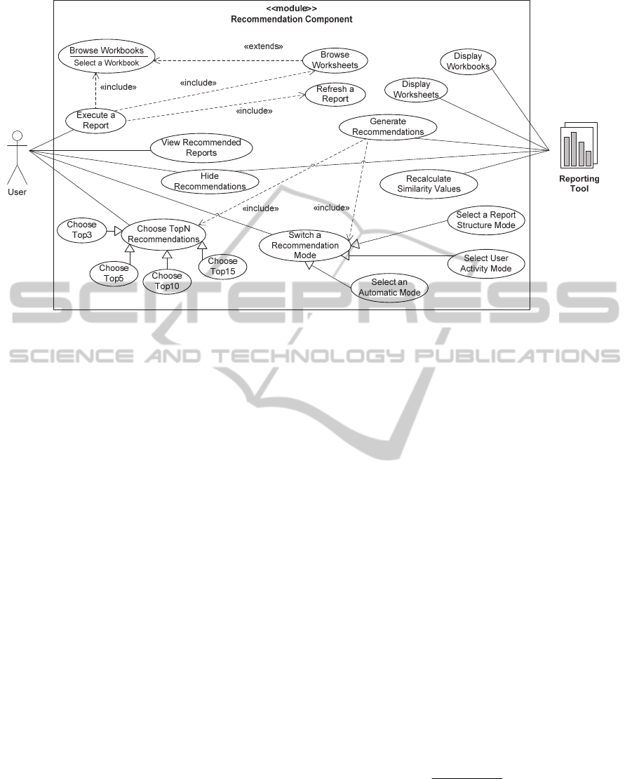
Figure 1: An UML Use Case diagram of the recommendation component of the data warehouse reporting tool.
user receives recommendations as in report structure
mode until crossing a threshold, and then – the user
activity mode is employed. A threshold, in fact, is a
borderline between the two modes. It is defined as a
positive constant, which represents the number of
records in the log belonging to a certain user, and is
considered to be sufficient to switch from one mode
to another. Threshold value is a subject to discuss
because of various factors that might affect it, e.g.,
the overall number of reports in the reporting tool,
the number of users, the number of available
reports, the overall volume of data warehouse, etc.
One should choose a threshold value taking into
consideration peculiarities of a particular data
warehouse and its reports. For instance, in our case,
a threshold value is equal to the number of distinct
workbooks that are accessible for each user. It is
presumed that by exploring each workbook in a time
period not exceeding three months the user is at
least acquainted with the reports (i.e. worksheets)
and its structure.
The hot-start method is composed of two main
steps. Firstly, user preferences for data warehouse
schema elements are discovered from the history of
user’s interaction with the reporting tool. Secondly,
reports that are composed of data warehouse schema
elements, which are potentially the most interesting
to a user, are determined.
We introduce weight to each element of a data
warehouse schema and a schema itself. Formal
description of weight assignment is given in
(Kozmina and Solodovnikova, 2011). Then, we
maintain and update the degree of interest (DOI) in
OLAP preferences by analyzing user behaviour in
the reporting tool employing the algorithm
(implemented as PL/SQL procedures) that calculates
the DOI of all schema elements and aggregate
functions.
In our approach one can distinguish two types of
DOI: (i) report degree of interest – the DOI of
elements of each report, and (ii) user profile degree
of interest – the DOI of all OLAP schema elements
detected in the user activity log. Afterwards, user’s
OLAP preferences are compared with OLAP
schema elements used in each report to estimate the
hierarchical similarity between a user profile and a
report. To calculate the hierarchical similarity, the
formula used to compute the user-item similarity
score for items defined by a hierarchical ontology
(Maidel, 2010) was considered, adopted and
adjusted. Thus, the hierarchical similarity between a
report and a user profile is computed as a ratio of the
sum of OLAP schema elements’ DOI in the report
to the sum of all OLAP schema elements’ DOI in
the user profile as seen in formula 1:
m
j
j
n
i
i
GDOI
EDOI
sim
1
1
)(
)(
,
(1)
where E
1
,…,E
n
are schema elements used in the
report, and G
1
,…,G
m
are all schema elements of the
user profile. A more detailed description followed
ICEIS2013-15thInternationalConferenceonEnterpriseInformationSystems
172

by examples can be found in (Kozmina and
Solodovnikova, 2011).
In practice, there are two types of similarity
coefficient calculated: fact-based (i.e., value of
hierarchical similarity is calculated for each report
for measures, fact tables and schemas) and
dimension-based (i.e., for attributes, hierarchies,
dimensions and schemas). It has been decided to
distinguish two types of similarity coefficients due
to the well-known characteristics of the data stored
in data warehouses, i.e., quantifying (measures) and
qualifying (attributes). However, the essence of any
data warehouse is in facts, while the describing
attributes give the auxiliary information. Thereby,
the recommendations are filtered (i) firstly, by the
value of the fact-based similarity coefficient, (ii)
secondly, by the one of dimension-based similarity
coefficient, and (iii) finally, by aggregate function
DOI.
Recommendations generated in Activity mode
for one of the reports – Total monthly students’
grade count by course (i.e, Kopējais vērtējumu
skaits mēnesī pa kursiem) – are presented in Figure
2. The usage scenario includes 10 recommendations
sorted in descending order, first, by the fact-based
similarity coefficient value, then, by the dimension-
based similarity coefficient, and finally, by
aggregate function DOI. As fact-based and
dimension-based similarity coefficient values may
highly differ, they are both shown to the user, for
instance, to make him/her aware of high extent of
dimension-based similarity even if the fact-based
similarity is average (e.g., reports #1: Monthly
distribution of students’ grade types by course, #3:
Total monthly grade count by course and by
professor, #4: Total monthly students’ final grade
count by course, #5: Total monthly students’ interim
grade count by course, and #6: Total monthly
students’ grade count by course) or low (e.g.,
reports #7: Gradebook usage by course, #9:
Students’ tasks by course, and #10: Total monthly
students’ task count by course and by professor).
The rest of the examples are with average fact-based
similarity and low dimension-based similarity
(report #2: Monthly distribution of students’ grade
types by study program) and low values of both
fact-based and dimension-based similarities (report
#8: Gradebook usage by course category).
In its turn, aggregate function DOI coefficient is
hidden from the user as it is considered to be less
informative but helpful in sorting in case when two
or more reports have same fact-based and
dimension-based similarity coefficient values, e.g.,
reports #4–#6 have equal fact-based and dimension-
based similarity values (respectively, 0.512; 0.679).
Such coefficient values illustrate that all three
reports consist of logical metadata with similar total
DOI value, whereas restrictions on data in these
reports may vary.
The cold-start method is composed of two steps:
(i) performance of structural analysis of existing
reports, and (ii) revealing likeliness between pairs of
reports. To be more precise, a pair of reports
consists of the report executed by the user at the
moment, and any other report which the user has a
right to access.
Here the report structure means all elements of
the data warehouse schema (e.g., attribute, measure,
fact table, dimension, hierarchy), schema itself, and
acceptable aggregate functions, which are related to
items of some report. In terms of structural analysis,
each report is represented as a Report Structure
Vector (RSV). In its turn, each coordinate of the
RSV is a binary value that indicates presence (1) or
absence (0) of the instance of the report structure
element. For example, in a RSV of a report Total
monthly grade count by course and by professor the
only element instances that are marked with 1 are:
attributes Month, Course, and Professor, measure
Grade count, dimensions Time, Course, and
Person,
fact table Students’ grades, schema Gradebook, and
aggregate function SUM. All the rest element
instances are marked with 0. Note that all report
structure elements are ordered the same way in all
reports. In case if any kind of change occurs, for
instance, a report is altered or a new report is
created, RSV of each report should be created all
over again.
To reveal likeliness between pairs of reports by
calculating the similarity coefficient, it is offered to
make use of Cosine/Vector similarity. It was
introduced by (Salton & McGill, 1983) in the field
of information retrieval to calculate similarity
between a pair of documents by interpreting each
document as a vector of term frequency values.
Later it was adopted by (Breese et al., 1998) in
collaborative filtering with users instead of
documents, and items’ user rating values instead of
term frequency values.
In recommender systems literature
Cosine/Vector similarity is extensively used
(Vozalis and Margaritis, 2004); (Rashid et al.,
2005); (Adomavicius et al., 2011), etc. to compute a
similarity coefficient for a pair of users in
collaborative filtering, or items in content-based
filtering. So, Cosine/Vector similarity of a pair of
AddingRecommendationstoOLAPReportingTool
173
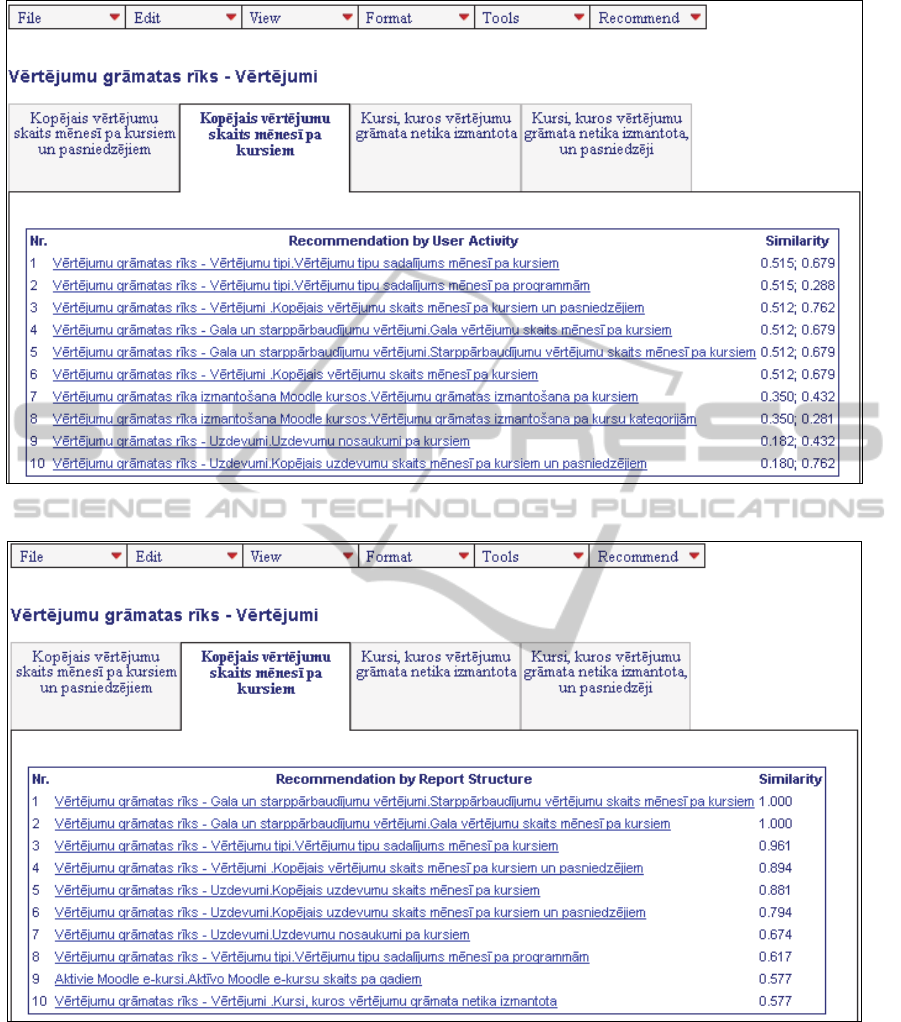
Figure 2: An example for recommendations in Activity mode (report Total monthly students’ grade count by course).
Figure 3: An example of recommendations in Structure mode (report Total monthly students’ grade count by course).
vectors is calculated. Examples of the RSV, its more
detailed description and calculation of the similarity
coefficient can be observed in (Kozmina and
Solodovnikova, 2011).
In the same way as described were the
recommendations in Structure mode generated for
one of the reports of the reporting tool – Total
monthly students’ grade count by course (i.e,
Kopējais vērtējumu skaits mēnesī pa kursiem). The
usage scenario that includes 10 recommendations
sorted by the similarity coefficient value in
descending order is depicted in Figure 3.
Note that reports #1: Total monthly students’
interim grade count by course and #2: Total monthly
ICEIS2013-15thInternationalConferenceonEnterpriseInformationSystems
174

students’ final grade count by course have the
similarity coefficient value equal to 1, which in its
turn means that the structure of these reports is the
same (i.e., the same OLAP schema elements are
employed). However, in case of high value of
similarity coefficient the data still may differ
because of various restrictions on data in each of
these reports. Also, if synonymic terms that denote
the semantic meaning of one and the same OLAP
schema element are different, it will not affect the
result (i.e., reports containing the same OLAP
schema elements will still have the similarity
coefficient value equal to 1).
The extent of similarity of each report in the
Top10 list and the one browsed by user at the
moment varies from high (1.000) to medium
(0.577). The higher the value of similarity
coefficient is (as in #1: Total monthly students’
interim grade count by course, #2: Total monthly
students’ final grade count by course, #3: Monthly
distribution of students’ grade types by course, #4:
Total monthly grade count by course and by
professor, and #5: Total monthly students’ task
count by course), the more the structure of these
reports is alike (i.e., the major part of OLAP schema
elements employed are the same). Naturally, lower
value of similarity coefficient (as in #9: Total yearly
active Moodle course count, and #10: Courses in
which gradebook is not being used) means the
opposite. Average similarity values are represented
by reports #6: Total monthly students’ task count by
course and by professor, #7: Students’ tasks by
course, #8: Monthly distribution of students’ grade
types by study program.
Executing (or refreshing) the recommended
report, a user receives another set of
recommendations (Generate Recommendations,
View Recommended Reports), and so on. The
maximum number of recommendations (Choose
TopN Recommendations) by default is 3 (Choose
Top3), but the user may adjust it to his/her taste to 5
(ChooseTop5), 10 (Choose Top10), or (Choose
Top15). If the user is convinced that
recommendations are not needed at the moment,
then he/she can turn this option off (Hide
Recommendations). All recommendation mode
settings are being saved and retrieved next time
when the user logs into the system.
Due to the fact that (i) a new report might be
created, (ii) there might be changes in existing
reports’ structure, or (iii) user’s activity during
preceding sessions should be analyzed, values of all
similarity coefficients have to be recalculated
(Recalculate Similarity Values). For now, it is
implemented as a maintenance procedure that is
being launched dynamically each time when a user
signs in or when some changes take place.
5 CONCLUSIONS AND FUTURE
WORK
In this paper a reporting tool developed and
currently being used at the University was briefly
described, however, an emphasis was placed on its
the recommendation component of this reporting
tool. A model to expose main user and system
activities was presented. Methods that were used in
all recommendation modes for generating
recommendations for reports were recalled.
Different usage scenarios of the recommendation
component applied to real data warehouse reports on
learning process were presented.
Naturally enough, it is planned to make some
experiments to test all three recommendation modes
(i.e., report structure mode, user activity mode, and
automatic mode) on a set of users. A possible
approach for validating recommendations as
interesting/uninteresting could be binary ratings – 1,
if the user visited the link on recommended report,
and 0 in the opposite case. Then, being guided by a
“precision/recall” technique – for instance,
presented in (Makhoul et al., 1999) – and having the
count of true-positive (recommended, selected),
false-positive (recommended, not selected), false-
negative (not recommended, selected), and true-
negative (not recommended, not selected), certain
parameters (i.e., precision, recall, false-positive rate)
that characterize the quality of recommendation are
calculated.
In one of our previous works (Kozmina and
Solodovnikova, 2012) a way for a user to create
OLAP preferences on the semantic level of metadata
– i.e., using description in business language:
operating with terms, its synonyms, and choosing
the most appropriate ones – was set forth. Thus, as
some of the future work the recommendation
component may be supplemented with one more
mode which is the option to state user preferences
explicitly by means of business language with the
following processing of such preferences and
generating recommendations based on them. For
that purpose the existing methods (i.e., hot-start and
cold start) of generating recommendations for
reports may be reconsidered, adopted and adjusted.
AddingRecommendationstoOLAPReportingTool
175

ACKNOWLEDGEMENTS
This work has been supported by the European
Social Fund within the project “Support for Doctoral
Studies at University of Latvia”.
REFERENCES
Adomavicius G., Manouselis N., Kwon Y.-O. 2011.
Multi-Criteria Recommender Systems. In: Ricci F, et
al. (eds) Recommender Systems Handbook, Springer,
Springer Science+Business Media, Part 5, pp 769-803
Aissi S., Gouider M.S. 2012. Towards the Next
Generation of Data Warehouse Personalization
System: A Survey and a Comparative Study.
International Journal of Computer Science Issues
(IJCSI), 9(3-2):561-568
Breese J.S., Heckerman D., Kadie C. 1998. Empirical
Analysis of Predictive Algorithms for Collaborative
Filtering. In: Proc. of 14th Conference on Uncertainty
in Artificial Intelligence (UAI'98), Madison, WI,
USA, pp 43-52
Garrigós I., Pardillo J., Mazón J.N., Trujillo J. 2009. A
Conceptual Modeling Approach for OLAP
Personalization. In: Laender, A.H.F. (ed.) ER 2009.
LNCS, Springer, Heidelberg, 5829:401-414
Giacometti A., Marcel P., Negre E., Soulet A. 2009.
Query Recommendations for OLAP Discovery Driven
Analysis. In: Proc. of 12th ACM Int. Workshop on
Data Warehousing and OLAP (DOLAP'09), Hong
Kong, pp 81-88
Golfarelli M., Rizzi S. 2009. Expressing OLAP
Preferences. In: Winslett, M. (ed.) SSDBM 2009.
LNCS, Springer, Heidelberg, 5566:83-91
Jerbi H., Ravat F., Teste O., Zurfluh G. 2009. Preference-
Based Recommendations for OLAP Analysis. In:
Proc. of 11th Int. Conf. on Data Warehousing and
Knowledge Discovery (DaWaK'09), Linz, Austria, pp
467-478
Kozmina N., Niedrite L. 2010. OLAP Personalization
with User-Describing Profiles. In: Forbrig P, Günther
H (eds.) BIR 2010. Springer, Heidelberg, LNBIP,
64:188-202
Kozmina N., Niedrite L. 2011. Research Directions of
OLAP Personalizaton. In: Proc. of 19th Int. Conf. on
Information Systems Development (ISD'10), Springer
Science+Business Media, pp 345-356
Kozmina N., Solodovnikova D. 2011. On Implicitly
Discovered OLAP Schema-Specific Preferences in
Reporting Tool. In: Scientific Journal of Riga
Technical University, Computer Science: Applied
Computer Systems, 46:35-42
Kozmina N., Solodovnikova D. 2012. Towards
Introducing User Preferences in OLAP Reporting
Tool. In: Niedrite L, et al. (eds.) BIR 2011
Workshops. Springer, Heidelberg, LNBIP 106:209-
222
Koutrika G., Ioannidis Y. E. 2004. Personalization of
Queries in Database Systems. In: Proc. of 20th Int.
Conf. on Data Engineering (ICDE'04), Boston, MA,
USA, pp 597-608
Maidel V., Shoval P., Shapira B., Taieb-Maimon M. 2010.
Ontological Content-based Filtering for Personalised
Newspapers: A Method and its Evaluation. Online
Information Review, 34(5):729-756, available online:
http://www.emeraldinsight.com/journals.htm?issn=14
68-4527&volume=34&issue=5
Makhoul J., Kubala F., Schwartz R., Weischedel R. 1999.
Performance Measures for Information Extraction. In:
Proc. of DARPA Broadcast News Workshop, Herndon,
VA, USA, pp 249-252
Mansmann S., Scholl M.H. 2007. Exploring OLAP
Aggregates with Hierarchical Visualization
Techniques. In: Proc. of 22nd Annual ACM
Symposium on Applied Computing (SAC'07),
Multimedia & Visualization Track, Seoul, Korea, pp
1067-1073
Marcel P., Negre E. 2011. A Survey of Query
Recommendation Techniques for Data Warehouse
Exploration. In: 7èmes journées francophones sur les
Entrepôts de Données et l'Analyse en ligne (EDA'11),
Clermont-Ferrand, France, B-7:119-134
Rashid A.M., Karypis G., Riedl J. 2005. Influence in
Ratings-Based Recommender Systems: An Algorithm-
Independent Approach. In: Proc. of 5th SIAM Int.
Conf. on Data Mining, Newport Beach, CA, USA, pp
556-560
Salton G., McGill M. 1983.
Introduction to Modern
Information Retrieval. McGraw-Hill Inc., New York,
NY, USA.
Solodovnikova D. 2007. Data Warehouse Evolution
Framework. In: Proc. of Spring Young Researcher's
Colloquium on Database and Information Systems
(SYRCoDIS'07), Moscow, Russia, available online:
http://ceur-ws.org/Vol-256/submission_4.pdf
Vozalis E., Margaritis K.G. 2003. Analysis of
Recommender Systems Algorithms. In: Proc. of 6th
Hellenic European Conference on Computer
Mathematics and its Applications (HERCMA'03),
Athens, Greece, pp 732-745
Vozalis M., Margaritis K.G. 2004. Enhancing
Collaborative Filtering with Demographic Data: The
Case of Item-based Filtering. In: Proc. of 4th Int.
Conf. on Intelligent Systems Design and Applications
(ISDA'04), Budapest, Hungary, pp 361-366.
ICEIS2013-15thInternationalConferenceonEnterpriseInformationSystems
176
