Isotropy Analysis of Optical Mouse Array for Mobile
Robot Velocity Estimation
Sungbok Kim
Hankuk University of Foreign Studies, Department of Digital Information Engineering,
Cheoin-gu, Yongin-si, Gyunggi-do, 449-791, Korea
Keywords: Optical Mice, Mobile Robot, Velocity Estimation, Isotropic Placement, Optimal Characteristic Length.
Abstract: This paper presents the isotropic analysis of an optical mouse array for the velocity estimation of a mobile
robot. It is assumed that there can be positional restriction on the installation of optical mice at the bottom of
a mobile robot. First, the velocity kinematics of a mobile robot with an array of optical mice is obtained, and
the resulting Jacobian matrix is analyzed symbolically. Second, the isotropic, anisotropic, and singular
optical mouse placements are identified, along with the corresponding characteristic lengths. Third, the least
squares mobile robot velocity estimation from the noisy optical mouse velocity measurements is discussed.
Finally, simulation results for the isotropic placement of three optical mice are given.
1 INTRODUCTION
For the velocity estimation of a mobile robot, several
attempts have been made to use optical mice that
were originally invented as an advanced computer
pointing device. In fact, an optical mouse is an
inexpensive but high performance motion detection
sensor with a sophisticated image processing engine
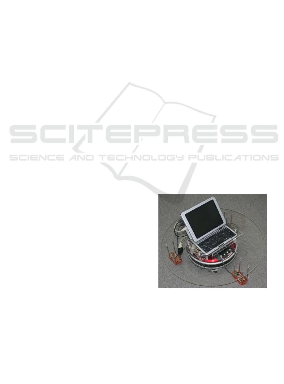
inside. Optical mice installed at the bottom of a
mobile robot, as shown in Fig. 1, can detect the
motions of a mobile robot traveling over a plane
surface. The mobile robot velocity estimation using
optical mice is free from the problems of typical
sensors: wheel slip in encoders, the line of sight in
ultrasonic sensors, and heavy computation in
cameras.
A pair of optical mice was proposed as a simple
but viable means for the mobile robot velocity
estimation in the presence of wheel slip (Lee and
Song, 2004; Bonarini et al., 2004). Using redundant
velocity measurements of two optical mice, a simple
procedure for error detection and reduction in the
mobile robot velocity estimation was developed
(Bonarini et al., 2005). The redundant number of
optical mice was proposed to reduce the effect of the
noisy velocity measurements of optical mice and to
handle their partial malfunction (Kim and Lee,
2008). Using the geometrical relationship among
optical mice, the calibration for systematic errors
and the selection of reliable velocity measurements
were presented (Hu et al., 2009).
Figure 1: A prototype of three optical mouse array for the
mobile robot velocity estimation (Kim and Lee, 2008).
For a mobile robot with a circular base, a regular
polygonal array of optical mice can be a natural and
desirable choice of the optical mouse placement. For
instance, a pair of optical mice are placed to be
symmetric about the center of a mobile robot. And,
3 optical mice are placed in a regular -gonal
array with its geometrical center coincident with the
center of a mobile robot (Kim and Lee, 2008).
However, there can be some restriction on the
installation of optical mice, owing to a non-circular
169
Kim S..
Isotropy Analysis of Optical Mouse Array for Mobile Robot Velocity Estimation.
DOI: 10.5220/0004435401690176
In Proceedings of the 10th International Conference on Informatics in Control, Automation and Robotics (ICINCO-2013), pages 169-176
ISBN: 978-989-8565-71-6
Copyright
c
2013 SCITEPRESS (Science and Technology Publications, Lda.)
base of a mobile robot or other structures pre-
installed on its base. With positional restriction on
installation, a non-regular polygonal array of optical
mice can be a better choice, compared with its
regular polygonal counterpart (Cimino and Pagilla,
2011).
The performance of an optical mouse array for
the mobile robot velocity estimation can be
evaluated based on its Jacobian matrix. The Jacobian
matrix maps the velocity of a mobile robot to the
velocities of optical mice, which is a function of the
installation positions of optical mice. Through the
Jacobian matrix, the unit sphere in the optical mouse
velocity space can be mapped into an ellipsoid in the
mobile robot velocity space. For the optimal
placement of optical mice, the volume of the
ellipsoid can be one measure, and also its closeness
to a sphere, so-called the isotropy, can be another
measure. The concept of isotropy has been adopted
for the optimal design of serial and parallel
manipulators (Ranjbaran et al., 1995; Angeles, 1997;
Chablat and Angeles, 2002; Zanganeh and Angeles,
1997; Fattah and Ghasemi, 2002), as well as,
omnidirectional mobile robots (Saha et al., 1995;
Kim and Moon, 2006).
This paper presents the isotropy analysis of an
optical mouse array for the mobile robot velocity
estimation. It is assumed that there can be positional
restriction on the installation of optical mice at the
bottom of a mobile robot. This paper is organized as
follows. Section 2 obtains the velocity kinematics of
a mobile robot equipped with optical mice, and
Section 3 analyzes the resulting Jacobian matrix
symbolically. Sections 4, 5, and 6 identify the
isotropic, anisotropic, and singular optical mouse
placements, along with the corresponding
characteristic lengths. Section 7 discusses the least
squares mobile robot velocity estimation from the
noisy optical mouse velocity measurements. Section
8 gives simulation results for the isotropic placement
of three optical mice. Finally, the conclusion is made
in Section 9.
2 VELOCITY KINEMATICS
The velocity of a mobile robot traveling on a plane
can be estimated using the velocity measurements of
2 optical mice installed at the bottom of a
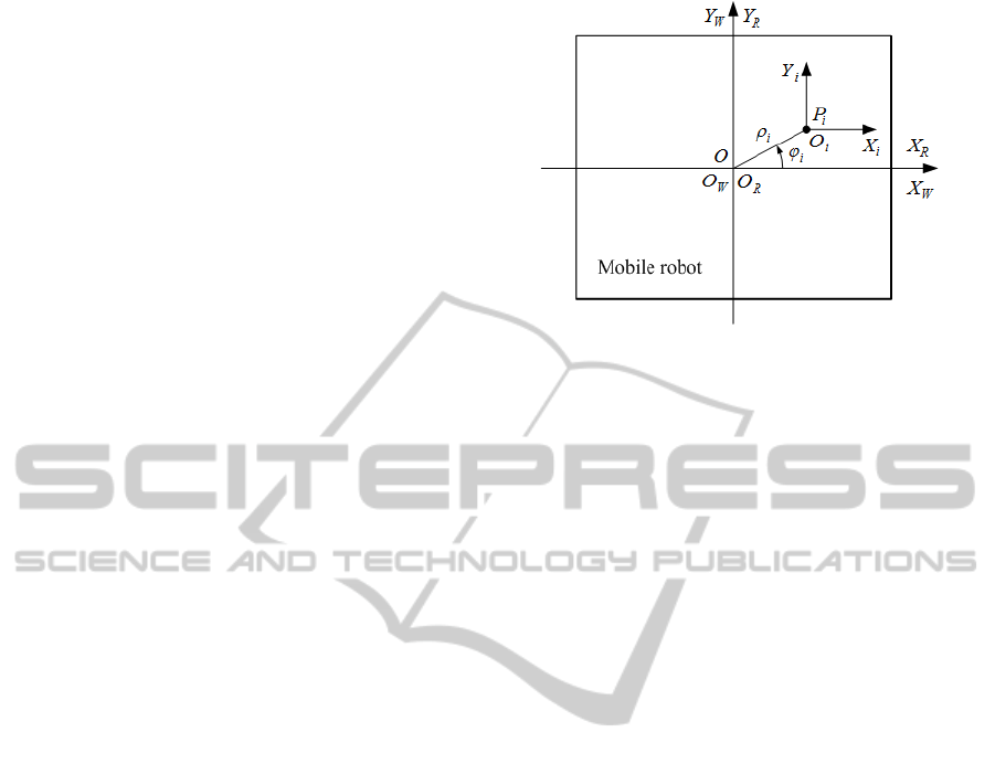
mobile robot. Fig. 2 shows three coordinate frames
that are used for the description of a mobile robot
and the
optical mouse. Let
,
, and
denote the origin, the and axes of the world
coordinate frame, respectively; let
,
, and
Figure 2: Three coordinate frames for a mobile robot and
the
optical mouse.
denote the origin, the and axes of the mobile
robot coordinate frame, respectively; and, let
,
,
and
, 1,⋯,, denote the origin, the and
axes of the
optical mouse coordinate frame,
respectively. For simple description, the following
assumptions are made. 1) Two origins,
and
,
are coincident with the center, denoted by , of a
mobile robot. 2) The origin,
, 1,⋯, is
coincident with the installation position,
, of the
optical mouse. 3) The world coordinate frame is
aligned with the mobile robot coordinate frame, with
which the
optical mouse coordinate frame is also
aligned. The position vector, p
,
1,⋯,, of the
optical mouse can be expressed
by
p
cos
sin
, 1,⋯,
(1)
where
and
are the polar coordinates of the
installation position
of the
optical mouse.
Let
and
be two linear velocity
components of a mobile robot long the axis and
the axis, respectively, and
be its angular
velocity component about the center of a mobile
robot. And, let that
and
,1,⋯,,be the
lateral and longitudinal velocity measurements of
the
optical mouse. The velocity relationship
between a mobile robot and the
optical mouse
can be presented by
, 1,⋯,
(2)
, 1,⋯,
(3)
From (2) and (3), the velocity kinematics of a
mobile robot with an array of optical mice can be
obtained by
A
(4)
In the above, v
∈
represents
the velocity vector of a mobile robot,
ICINCO2013-10thInternationalConferenceonInformaticsinControl,AutomationandRobotics
170

⋯
∈
represents the velocity
vector of optical mice, with
,
1,⋯, being the velocity measurement of the
optical mouse; and, represents the Jacobian matrix
mapping
to
, given by
1
0
1
0
⋮
1
0
0
1
0
1
⋮
0
1
⋮
∈R
(5)
Note that the expression of is very simple as a
function of the positions of optical mice, p
, 1,⋯,.
3 SYMBOLIC ANALYSIS
In the velocity kinematics of (4), the velocity vector
of a mobile robot,
is composed of two linear and
one angular components, while the velocity vector
of optical mice,
, is composed of a total of 2
linear components. To eliminate the physical
inconsistency among velocity components, the
characteristic length, denoted by , can be
introduced (Angeles, 1997):
(6)
where
∈
and
10
1
0 1
1
10
1
0 1
1
⋮ ⋮ ⋮
10
1
0 1
1
∈R
(7)
Note that all elements of
are physically
dimensionless.
From (7),
can be written as
10
01
∈R
(8)
where
1
(9)
1
(10)
1
1
(11)
In the above,
and
, respectively, represent the
averages of the and coordinates of the position
vectors, p
, 1,⋯,, of optical
mice, and represents the root mean square of the
distances of optical mice from the center of a
mobile robot.
Using (8), the characteristic polynomial of
is given by
1
0
(12)
From (12), three eigenvalues of
, denoted by λ
,
λ
, and λ
, are obtained by
λ
2
1
1
4
(13)
λ
(14)
λ
2
1
1
4
(15)
It can be shown that there hold the following
inequality relationships among three eigenvalues, λ
,
λ
, and λ
:
(16)
regardless of the values of C
, C
, and
, as well as
. Note that λ
and λ
are the largest and smallest
eigenvalues of
, while λ
is its middle
eigenvalue which remains constant as .
IsotropyAnalysisofOpticalMouseArrayforMobileRobotVelocityEstimation
171

4 ISOTROPIC PLACEMENT
For the 23 Jacobian matrix
with 2, the
condition number can be defined by
(17)
where
and
represent, respectively, the largest
and smallest singular values of
, and λ
and λ
represent, respectively, the largest and smallest
eigenvalues of
. Note that the condition number
can have values from unity to infinity. The
Jacobian matrix
is isotropic when 1, and
is
singular when ∞.
The placement of optical mice is said to be
isotropic, if the isotropy of the 23 Jacobian
matrix
can be achieved:
(18)
where
represents that 33 identity matrix. Note
that
has three identical eigenvalues of
magnitude , that is, λ
λ
λ
, so that the
condition number becomes unity, 1. From (8)
and (18), the isotropy conditions for
are given by
1
0
(19)
1
0
(20)
1
1
1
(21)
In the above, (19) and (20) indicate that the
geometrical center of optical mice coincides with
the center of a mobile robot. And, (21) indicates
that the squared value of the characteristic length
should be equal to the average of the squared
distances of optical mice from the center .
Using (1), (19), and (20) can be written as:
0
(22)
Let
be the isotropic set of the position vectors of
optical mice, satisfying (22):
,1,⋯,
0
(23)
For given
2
optical mice, Fig. 3 shows the
isotropic sets of position vectors,
,1,⋯,.
In the case of 2 shown in Fig. 3(a), the
isotropic set
can be parameterized by two
(a) (b)
(c)
(d)
Figure 3: The isotropic set of the position vectors of
optical mice: (a) 2, (b) 3, (c) 4, and (d)
4.
variables,
,
; in the case of 3 shown in Fig.
3(b), the isotropic set
can be parameterized by
four variables,
,
,
,
; and, in the case of
4 shown in Figs. 3(c) and 3(d), the isotropic
set
can be parameterized by 21 variables,
,
,
,⋯,
,
,
. Note that the rotation
of the isotropic set of position vectors by the angle
with respect to the center of a mobile robot are
also isotropic:
Since the union of two isotropic sets is also
isotropic, new isotropic sets for 4 position
vectors can be obtained from existing isotropic sets
known already:
⋃
(24)
where
, 2
,
2. For
5 optical mice, Fig. 4(a) shows the isotropic set
, which is obtained as the union of
and
.
However, note that (24) cannot produce all possible
isotropic sets of position vectors, since
∑
∑
0 is sufficient but not necessary for
∑
0. It should be mentioned that the
simplest isotropic set of position vectors is a
regular polygon, for which
⋯
(25)
⋯
360°
(26)
ICINCO2013-10thInternationalConferenceonInformaticsinControl,AutomationandRobotics
172

Fig. 4(b) shows the isotropic placement of =5
optical mice, which from a regular pentagon.
Once the isotropic placement of optical mice,
denoted by
∗
∗
∗
, 1,⋯,, is
determined from (19) and (20), the value of the
characteristic length , required for the isotropy of
the Jacobian matrix
, can be determined, from (21):
(a)
(b)
Figure 4: Two isotropic sets of 5 position vectors: (a)
∪
, and (b) a regular pentagon.
∗
∗
1
∗
∗
(27)
which is called as the optimal characteristic length.
Note that the optimal characteristic length
∗
is the
root mean square of the distances of position
vectors,
∗
,1,⋯,, from the center O of a
mobile robot.
5 ANISOTROPIC PLACEMENT
For a given placement of optical mice, it may be
impossible to achieve the isotropy of the 23
Jacobian matrix
. Seen from (15), the smallest
eigenvalue of
, λ
, can be zero, and thus we
consider the condition index, defined by
λ
λ
(28)
which is the inverse of the condition number of
, given by (17). Note that the condition index
can have values between zero and unity, where
is isotropic when 1, and
is singular when
0. For the placement of optical mice, it is
desirable to make the value of as large as possible.
Using (13) and (15), (28) can be written as
√
√
(29)
with
1
(30)
1
4
(31)
Setting
equal to zero, we have
2
(32)
with
2
(33)
4
8
(34)
Plugging (30), (31), (33), and (34) into (32), it
follows that
0
(35)
As will be shown later,
(36)
unless
is singular. From (35) and (36), using
(11), the condition for maximizing the value of is
obtained by
0
(37)
which results in
#
#
1
(38)
which is called as the suboptimal characteristic
length. It should be noted that the expression of the
suboptimal characteristic length
#
, given by (38), is
the same as that of the optimal characteristic length
∗
, given by (27).
With the suboptimal characteristic length
#
known, the maximum value of the condition index
that can be achieved for a given anisotropic optical
mouse placement can be obtained. Plugging (37) and
(38) into (30) and (31) and using (29), we obtain
#
#
#
(39)
which is called as the maximal condition index. Note
that the maximal condition index
#
can have values
between zero and unity, where
#
1 when
0, and
#
0 when
#
#
.
IsotropyAnalysisofOpticalMouseArrayforMobileRobotVelocityEstimation
173

6 SINGULAR PLACEMENT
The placement of optical mice is said to be
singular, if
falls into singularity, that is, the
smallest eigenvalue of
, λ
, becomes zero:
λ
0
(40)
for which the condition index becomes zero, 0.
From (15) and (40), we have
1
1
4
(41)
which leads to
(42)
Plugging (9)-(11) into (42) and using (1), we have
1
2
cos
,
0
(43)
(43) can be rearranged into
2
cos
,
0
(44)
where
,
,
1,⋯,1,
,,
1
,⋯,
(45)
represents the angle between two position vectors,
and
, 1,⋯,1, 1,⋯,.
It can be shown that
0
2
cos
,
(46)
In the above, the equality holds, when cos
,
1
or cos
,
1, 1,⋯,1,
1,⋯,. In the former case, for which
,
0,
1,⋯,1,
1,⋯,
(47)
and, from (44), we have
0
(48)
which results in
⋯
(49)
Note that (47) and (49) indicate that optical mice
are placed at the same position on a mobile robot.
Next, in the latter case, for which
,
180
°
,
1,⋯,1,
1,⋯,
(50)
and, from (44), we have
0
(51)
which results in
⋯
0
(52)
(52) indicates that optical mice are placed at the
center of a mobile robot. At both singular
placements of optical mice, one given by (47) &
(49) and the other given by (52), it should be noted
that the rank of the Jacobian matrix
drops to two.
7 LEAST SQUARES VELOCITY
ESTIMATION
Based the velocity kinematics of (6), the mobile
robot velocity can be estimated from the noisy
velocity measurements
of optical mice by
(53)
where
∈
(54)
Note that (53) with (54) represents the least squares
solution to (6), which minimizes
.
Assume that the placement of optical mice is
isotropic, with the isotropic position vectors
∗
∗
∗
, 1,⋯,, and the optimal
characteristic length
∗
. Plugging (7), (18), and (27)
into (53), we have
1
1
0
∗
0
1
∗
1
0
∗
0
1
∗
⋯
⋯
⋯
1
0
∗
0
1
∗
(55)
Using (55), from (53), the estimated velocity of a
mobile robot is obtained by
ICINCO2013-10thInternationalConferenceonInformaticsinControl,AutomationandRobotics
174
1
(56)
1
(57)
1
(58)
where
1
∗
∗
∗
,
1,⋯,
(59)
represents the angular velocity component
experienced by the
optical mouse, which is
equivalent to the velocity measurement
,1,⋯,. Seen from (56)-(58), two
linear and one angular components of the esimated a
mobile robot velocity can obtained by the averages
of the corresponding components of optical mice.
Note that such a computational simplicity in the
mobile robot velocity estimation is attributed to the
isotropic placement of optical mice.
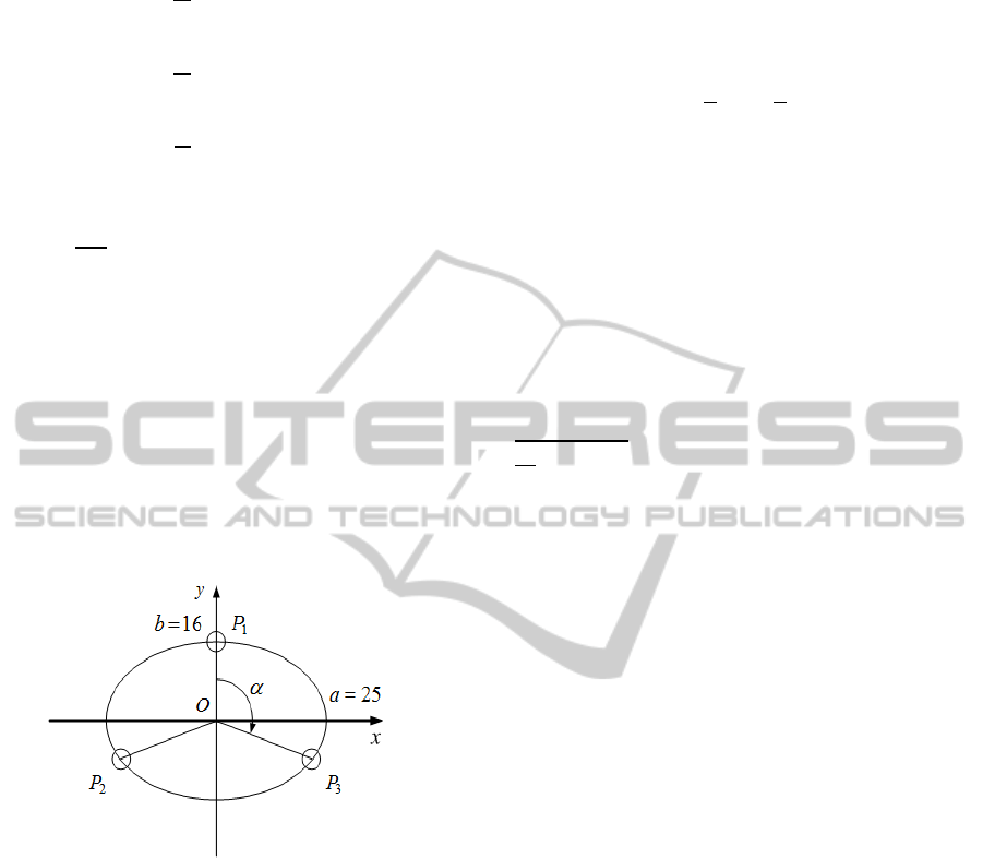
Figure 5: The symmetrical placement of three optical mice
along an elliptical path.
Now, let us discuss the role of the characteristic
length in the least squares mobile robot velocity
estimation, given by (53) with (54), which involves
the inversion of
. Seen from (8), it is apparent
that the selection of will affect the conditioning of
, for a given optical mouse placement,
,1,⋯,. For instance, if is chosen to
be too small,
becomes close to singularity. This
may lead to numerical instability during the
inversion process of
, so that the accuracy of the
estimated mobile robot velocity can be unacceptably
poor. On the other hand, the proper selection of ,
most preferably
#
, given by (39), can improve
the conditioning of
, even when a given optical
mouse placement is near singular.
8 SIMULATION RESULTS
Suppose that three optical mice(3) are placed
on an elliptical path, given by
,
|
1
(60)
where the first optical mouse is fixed on the
principal axis along the axis, but the second and
third optical mice that are symmetric with respect to
the axis, as shown in Fig. 5 where 25cm,
16cm, and 0°90°. Using (19) and (20),
the isotropic optical mouse placement can be found
at
∗
120°, corresponding to
∗
,
∗
,
∗
90°,210°,330°
. Note that three optical mice form
an equilateral triangle in general, but they will form
a regular triangle if the elliptical path becomes
circular, that is, . And, using (27), the optimal
characteristic length is obtained by
∗
20.99cm. On the other hand,
using (47) and (49), the singular optical mouse
placement can be found as
,
,
90°,90°,90°
.
Next, let us examine the least squares velocity
estimation of a mobile robot for a given placement
of three optical mice. Assume that a mobile robot is
commanded to move forward along the axis at the
velocity of
0cm/sec,
20cm/sec, and
0deg/sec. To simulate the noisy velocity
measurements of three optical mice, normally
distributed random numbers,
and
,1,2,3,
with mean 0 and variance 0.2 are added,
independently, to the nominal values of the and
velocity components of each optical mouse. With
0200
, using (4), the noisy velocity
measurements of three optical mice are obtained by
(61)
where
∈
with
,1,2,3, represents the random noise
vector experienced by three optical mice. For the
isotropic optical mouse placement, Fig. 6 shows the
velocity measurements of the first optical mouse, and
the resulting least squares velocity estimation of a
mobile robot, using (53) with (54). Note that a total of
10,000 samples are taken in our simulation, but for
better visibility, only 500 samples are plotted in Fig.
6. Overall, it can be observed that the effects of noisy
velocity measurements of three optical mice are
reduced significantly. The noise levels of two linear
components,
and
, of the estimated mobile
robot velocity amount to about 58% of those of two
linear velocity components of each optimal mouse.
IsotropyAnalysisofOpticalMouseArrayforMobileRobotVelocityEstimation
175
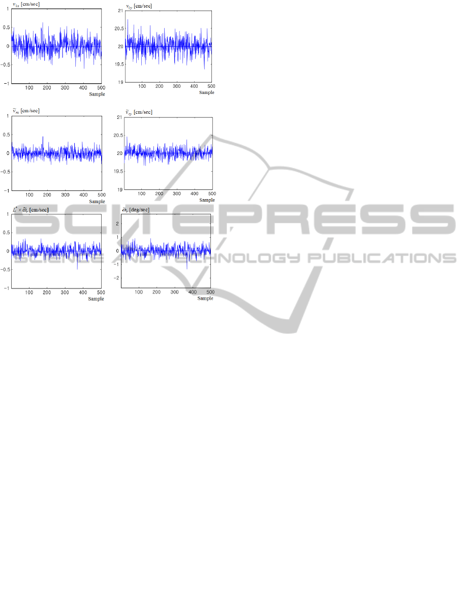
(a)
(b)
Figure 6: The least squares mobile robot velocity
estimation from the noisy optical mouse velocity
measurements: (a) the measured velocity components,
and
, and (b) the estimated velocity components,
,
,
∗
, and
.
9 CONCLUSIONS
In this paper, we presented the isotropy analysis of
an optical mouse array for the mobile robot velocity
estimation. Positional restriction on the installation
of optical mice at the bottom of a mobile robot is
assumed. The main contributions of this paper can
be summarized as 1) the symbolic analysis of the
Jacobian matrix, mapping the mobile robot velocity
to the optical mouse velocities, 2) the identification
of the isotropic, anisotropic, and singular optical
placements along with their corresponding
characteristic lengths, and 3) the application to the
least squares mobile robot velocity estimation from
the noisy optical mouse velocity measurements. The
results of this paper can be helpful especially for the
development of personal robot mobile platforms
having a non-circular base.
ACKNOWLEDGEMENTS
This work was supported by Hankuk University of
Foreign Studies Research Fund of 2013.
REFERENCES
Lee S. and Song J., Mobile Robot Localization Using
Optical Flow Sensors, In Int. J. Control, Automation,
and Systems, vol. 2, no. 4, pp. 485-493, 2004.
Bonarini A., Matteucci M., and Restelli M., A Kinematic-
independent Dead-reckoning Sensor for Indoor Mobile
Robotics, In Proc. IEEE Int. Conf. on Intelligent
Robots and Systems, pp. 3750-3755, 2004.
Bonarini, A., Matteucci M., and Restelli M., Automatic
Error Detection and Reduction for an Odometric Sensor
based on Two Optical Mice, In Proc. IEEE Int. Conf. on
Robotics and Automation, pp. 1687-1692, 2005.
Kim S. and Lee S., Robust Velocity Estimation of an
Omnidirectional Mobile Robot Using a Polygonal
Array of Optical Mice, In Int. J. Control, Automation,
and Systems, vol. 6, no. 5, pp. 713-721, 2008.
Hu J., Chang Y., and Hsu Y., Calibration and On-line Data
Selection of Multiple Optical Flow Sensors for
Odometry Applications, In Sensors and Actuators A,
vol. 149, pp. 74-80, 2009.
Cimino M. and Pagilla P. R., Optimal Location of Mouse
Sensors on Mobile Robots for Position Sensing, In
Automatica, vol. 47, pp. 2267-2272, 2011.
Ranjbaran F., Angeles J., Gonzalez-Palacios M. A., and
Patel R. V., The Mechanical Design of a Seven-Axes
Manipulator with Kinematic Isotropy, In J. of Intelligent
and Robotic Systems, vol. 12, pp. 21-41, 1995.
Angeles J., Fundamentals of Robotic Mechanical Systems,
Springer, 1997.
Chablat D. and Angeles J., On the Kinetostatic
Optimization of Revolute-Coupled Planar
Manipulators, In Mechanism and Machine Theory,
vol. 37, pp. 351-374, 2002.
Zanganeh K. E. and Angeles J., Kinematic Isotropy and the
Optimum Design of Parallel Manipulators, In Int. J. of
Robotics Research, vol. 16, no. 2, pp. 185-197, 1997.
Fattah A. and Ghasemi A. M. H., Isotropic Design of
Spatial Parallel Manipulators, In Int. J. of Robotics
Research, vol. 21, no. 9, pp. 811-824, 2002.
Saha S. K., Angeles J., and Darcovich J., The Design of
Kinematically Isotropic Rolling Robots with
Omnidirectional Wheels, In Mechanism and Machine
Theory, vol. 30, no. 8, pp. 1127-1137, 1995.
Kim S. and Moon B., Complete Identification of Isotropic
Configurations of a Caster Wheeled Mobile Robot
with Nonredundant/Redundant Actuation, In Int. J.
Control, Automation, and Systems, vol. 4, no. 4, pp. 1-
9, Aug. 2006.
ICINCO2013-10thInternationalConferenceonInformaticsinControl,AutomationandRobotics
176
