Viability Study on Supervisory Control for a Solar Powered Train

Beatriz F

eria and Jo

ao Sequeira

Instituto Superior T

ecnico/Institute for Systems and Robotics, Lisbon, Portugal

Keywords:

Solar Powered Train, Petri Nets, Supervisory Control, Energy Management System.

Abstract:

This paper addresses the design and simulation of a control system for a solar powered train. An intelligent

control approach using Petri nets is followed aiming at managing the energy consumption such that the train

always reaches its destination. The system uses a priori information on the topology of the line, including

length and slopes, locations of the intermediate stations, and also on the dynamics of the train, current solar

irradiance and weather forecasting, and passenger weight, to determine bounds on the train velocity proﬁle.

The whole system was simulated integrating Petri nets in a Matlab/Simulink environment.

1 INTRODUCTION

This paper describes ongoing work under the frame-

work of project Helianto (see (Helianto, 2013)) aim-

ing at designing a multi-purpose solar powered light

train. The paper describes a simulation environment

built to assess the viability of the project.

The Helianto solar train is an autonomous vehi-

cle, powered exclusively by solar energy and batter-

ies. This makes it attractive for touristic purposes,

connecting urban centers and environmentally sensi-

tive areas. The train is equipped with an array of so-

lar panels that can adjust their orientation in order to

maximize the solar energy captured. The batteries on-

board are recharged from the electric grid, whenever

the train stops at a station, and using energy regener-

ated from braking.

Energy management systems have been exten-

sively studied in a multitude of applications (Godoy

Simaes et al., 1998; Jinrui et al., 2006). Route topol-

ogy, predicted meteorological conditions and forces

opposing the motion, gravity, rolling resistance and

aerodynamic drag are examples on relevant condi-

tions for project design, (Godoy Simaes et al., 1998)

In order to develop the energy management system,

all the components dealing with energy onboard the

train and even those located on the outside, namely at

the stations and along the railway line have to be mod-

eled realistically. In the Helianto project, the over-

all system is modeled through discrete events sys-

tems (DES). DES have an elegant representation in

the form of Petri nets, for which there are available

powerful analysis tools (Moody et al., 1994; Davidra-

juh, 2008; G. Cassandras and Lafortune, 2008) and

for which supervisory controller design techniques al-

low an easy inclusion of constraints found in this type

of application. In a sense,this is also resource man-

agement problem and Petri nets are reference tools to

this class of problems, (Bogdan et al., 2006).

This paper is organized as follows. Sections 2 and

3 discuss some of the modeling options and simula-

tion tools. Section 4 presents a Petri net model of the

overall system, with the corresponding supervisory

controller being described in Section 5. Simulation

results are discussed in Section 6 and the conclusions

of the paper are presented in Section 7.

2 INFRASTRUCTURE

The topology of the line and the placement of the

stations placed along the line are assumed a priori

known. The train uses GPS and the information on

the topology of the line, eventually with a selection

of landmarks placed along the line. Standard robotic

sensors, e.g., laser range ﬁnders, can be used to detect

obstacles. Also, an internet connection can be used

to access short-term weather forecast services for the

region where the train is operating, if available.

Each station can be equipped with a gate through

which the passengers must go through to access the

train. The gate system keeps count on how many peo-

ple are in the station ready to board the train. More-

over, weight sensors at the gate ﬂoor allow to estimate

the total weight to board the train at each station.

423

Féria B. and Sequeira J..

Viability Study on Supervisory Control for a Solar Powered Train.

DOI: 10.5220/0004422404230430

In Proceedings of the 3rd International Conference on Simulation and Modeling Methodologies, Technologies and Applications (SIMULTECH-2013),

pages 423-430

ISBN: 978-989-8565-69-3

 2013 SCITEPRESS (Science and Technology Publications, Lda.)

Given a time schedule for the train, specifying the

arrival and departure times at each station, the goal

of the supervisory controller is to generate a velocity

proﬁle reference such that (i) the train complies with

the schedule, even in presence of abnormal events,

(ii) the use of energy from the battery set is mini-

mized, and (iii) the velocity and acceleration are al-

ways within operational limits deﬁned by passenger

comfort requirements. In case is not possible to ﬁnd a

solution the train must not start moving.

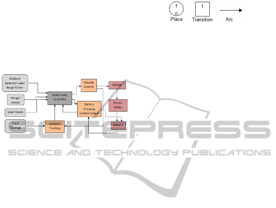
Figure 1: Block diagram of the overall system.

Figure 1 presents the block diagram for the global

system.

Since it is a low-speed train, skidding is neglected

and thus the dead-reckoning estimate can be fused,

in the ”Location Tracking” block, with GPS and

landmark information using standard Kalman ﬁlter-

ing techniques.

Once a reference velocity is generated by the cor-

responding block, the ”Vehicle” block communicates

to the ”Motor” block the necessary torque which in

turn generates the mechanical power required to move

the train.

The batteries are kept at all times within an admis-

sible range by the ”Battery charging control” block .

In case a minimum charge value is reached the block

prevents further discharging and signals the system

that the battery needs to be charged at the next sta-

tion.

3 SIMULATION ENVIRONMENT

The simulation tool was developed under the

Simulink environment with the toolboxes QSS, (QSS,

2008), to model the dynamics of the train, and Netlab,

(Netlab, 2008), to construct a Petri net model of the

system.

Netlab allows the design and graphical simulation

of Petri Nets and can also interface Matlab/Simulink.

Simulink imports a Netlab net as a single block. The

exchange of data between the Petri net and the rest

of the environment is reduced to the marking in input

and output places.

Figure 2: Netlab symbols for Petri nets.

Figure 2 illustrates the Netlab symbols used in the

Petri nets. Supervisory control is then applied to the

overall system through the Petri net block, establish-

ing a direct, real-time, communication with Simulink.

The QSS toolbox simulates the behavior of a vehi-

cle, motor and energy source, for given velocity and

acceleration proﬁles, accounting, among others, for

weight, wheel diameter, frontal area, friction and drag

coefﬁcients, and motor inertia. The velocity and ac-

celeration proﬁle is calculated based on information

from the location tracking block, panels, and sensors.

The track gradient proﬁle is deﬁned based on track

topology and location tracking block. These inputs

are assumed to be constant during each time interval,

which for the purpose of this work was set to 1 sec-

ond. At each step the torque required for the vehicle

to follow the speciﬁed velocity proﬁle is calculated,

together with the necessary energy.

4 PETRI NET MODEL

4.1 Train

Figure 3a shows the Petri net modeling this subsys-

tem. The main states are represented by places. A

single token is passed on from place to place repre-

senting the current situation of the train. Once the

train is ready, it starts moving when transition 1 is

triggered, representing a start command. While mov-

ing two events can occur, the train enters a station

(transition 5), or the laser detects an obstacle (transi-

tion 3). The ﬁrst leads the train to stop and remain on

a terminal state waiting to proceed to the next trunk.

The second also leads the train to stop and wait for

permission to ﬁnish the current trunk. These transi-

tions can be assumed non-conﬂicting without loosing

generality. In fact it is enough that obstacle detection

range is longer than the length of the station approach-

ing zone.

4.2 Motor

Figure 3b represents the Petri net that models the elec-

tric motor. There are four main operation modes for

the motor and each one is represented by a place. The

presence of a token in one of these places indicates the

current mode of the motor. Once the motor is started

SIMULTECH2013-3rdInternationalConferenceonSimulationandModelingMethodologies,Technologiesand

Applications

424

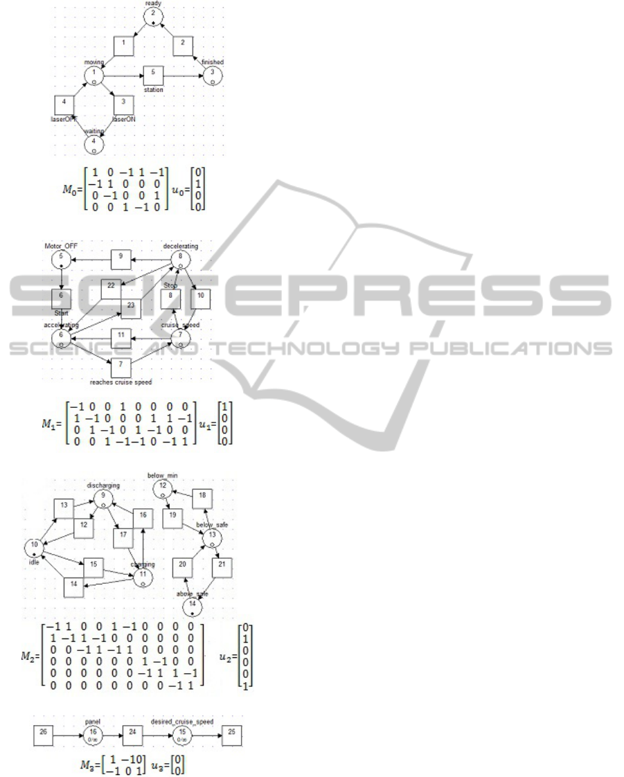
(a) Petri net train behavior model.

(b) Petri net motor behavior model.

(d) Petri net model for target velocity.

Figure 3: Petri net models for the main sub-systems and

respective incidence matrices and initial conditions.

(transition 6) it accelerates until the vehicle reaches

the referenced cruise velocity (transition 7). Once this

happens the motor switches to cruise velocity mode.

From this mode two possible events can occur: the

vehicle stops (transition 8), and in that case the mo-

tor switches to decelerating mode or the vehicle is al-

lowed to increase cruise velocity (transition 11) and

in that case it switches to accelerating mode. Tran-

sition 8 can be set by three different types of events.

The ﬁrst occurs when the train approaches a station,

then transition 8 ﬁres leading the motor to decelerate

until it stops. The second occurs when the laser range

ﬁnder detects an object. If this happens the train is

required to stop and transition 8 ﬁres leading the ve-

hicle to decelerate until it stops. In case the obstacle is

no longer detected (transition 22) it is possible for the

vehicle to switch from decelerating mode to accelerat-

ing mode in order to resume previous motion. Finally

transition 8 can also be set by a power decrease event.

If the output power of panels can no longer support

current cruise velocity, transition 8 ﬁres and the mo-

tor decelerates until a supported velocity is reached.

It is also possible that this situation is reversed. This

means that if the output power of panels increases,

so does the supported cruise velocity and the motor

switches to accelerating mode (transition 11) until it

reaches the new cruise velocity.

4.3 Battery

The battery is modeled according to the stages of op-

eration and the charge level condition (Figure 3c).

There are three possible stages of operation for the

battery: idle, charging and discharging. If the power

delivered by the panels is not enough to sustain min-

imum cruise velocity, the battery is allowed to dis-

charge the necessary power so that the vehicle reaches

that velocity. Also during accelerating mode, where a

power peak demand occurs, the battery is allowed to

discharge since the power requested during this mode

is higher than the panels can deliver. If none of these

situations occur, the battery remains in an idle stage

waiting for a discharging or charging request.

The battery enters charging mode whenever the

motor decelerates, through the regenerative braking

system or at the stations, through the power grid,

whenever the charge is below the safety value.

The battery condition is also modeled by three

main states: above safety value, below safety value

and below minimum value. The minimum value rep-

resents a characteristic property of each type of bat-

tery that states that the battery charge should never

cross that threshold, at the risk of malfunction.

The safe value represents the necessary charge

ViabilityStudyonSupervisoryControlforaSolarPoweredTrain

425

that ensures the train reaches the next station con-

sidering situations such as low irradiance, obstacles

on the track or even communication failure. At every

station this minimum value must be met, charging the

battery if necessary. If the battery charge remains be-

tween these two values, the token remains in the place

representing below safe state.

4.4 Cruise Speed Reference

Figure 3d deﬁnes the desired cruise speed for the ve-

hicle directly from the power delivered by the panels.

Through transition 26, the marking of place 16 rep-

resenting the panel is determined by Simulink. This

means that the number of tokens in place 16 corre-

sponds to the power delivered by the panels. The

transfer of real measurements into the Petri net re-

quires that those values are discretized and quantiﬁed

into tokens. For instance, 1 token in place 16 means

that the panels are delivering 1Kw power. The same

reasoning is applied to velocity which means that 1 to-

ken in place 15 corresponds to a speciﬁc value cruise

velocity for the vehicle. This calculation assumes

that speed varies linearly with power. This linearity

can actually be veriﬁed for low velocities such as the

range considered for the solar train, (Andr

e, 2006).

5 SUPERVISORY CONTROLLER

The subsystems in Figure 3, that form the Helianto

system are controlled by a supervisor, in charge of ac-

counting for the constraints related to the resources

and operation requirements. The approach followed

in this work is that in (Moody et al., 1994). Roughly,

it consists in describing the desired behavior for the

supervisor through a set of linear constraints involv-

ing the marking and transition vectors.

A ﬁrst version of the supervisor accounts for a ba-

sic set of constraints, listed below. This set does not

yet account for temporal constraints such as the train

timetable.

1. Once the battery crosses a minimum value thresh-

old it stops discharging.

2. While the battery remains under minimum charge

value, it cannot discharge.

3. The train is only allowed to begin traveling the

next trunk in case the battery charge is above the

safe value.

4. While the motor is at cruise speed mode it

switches to decelerating mode when a station ap-

proaches or an obstacle is detected.

Table 1: Algebraic constraints and controller solution; v

and u

stand for the values of transitions and place mark-

ings, respectively.

Constraint Description Additional

places

Additional

arcs

1 v

≤ v

place 19 –

2 u

+ u

≤ 1 place 18 –

3 v

≤ u

— 2

4 v

≤ u

– 4

5 v

≤ u

– 2

6 u

≤ 4 place 17 –

5. While the motor is off it only starts when the train

is set to begin the next trunk or when an obstacle,

causing the train to stop, is no longer detected.

6. Cruise speed cannot exceed a certain value.

The incidence matrix used corresponds to the global

system matrix,

M =







0 0 0

0 M

0 0

0 0 M

0 0 0 M







where M

and M

are deﬁned in Figure 3.

Table 1 summarizes the constraints as well as the

controller places and arcs, on Figure 4, that result

from each constraint.

The resulting supervised system is shown in Fig-

ure 4 where color (thick) arcs and places represent the

controller elements added to the baseline model.

Accounting for a timetable can be done in multiple

ways, e.g., (i) using a timed transition from place 7 to

a new place so that the elapsed time can be counted

through the marking of this new place, or (ii) simply

add a new input place with the marking being deﬁned

after the events generated according to a real clock

from Simulink. Each of these ways requires an ac-

tive changing of the constraint that bounds the cruise

velocity, in place 15, this meaning that a minimum

cruise must be deﬁned in order to the train meeting the

schedule. The second of the aforementioned strate-

gies was implemented and a new transition connected

to a new place were added to the model. Since Netlab

does not include timed transition elements, the transi-

tion is commanded by an external signal in Simulink

that allows the ﬁring whenever simulation time in-

creases by one second. Once the transition ﬁres a

token is placed in the new place in order to account

for the elapsed time. The same was applied to dis-

tance, and another transition and place were added to

the model with the purpose of counting the covered

distance. Both the covered distance and elapsed time

signals are transferred to Simulink so that a minimum

cruise velocity is deﬁned for the train on a real-time

basis.

SIMULTECH2013-3rdInternationalConferenceonSimulationandModelingMethodologies,Technologiesand

Applications

426

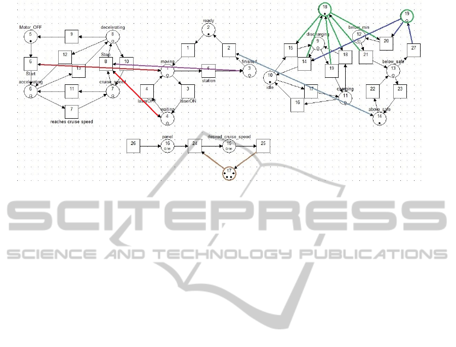
Figure 4: Petri net model of the supervised system.

6 SIMULATION RESULTS

This section presents simulation results obtained for

the model designed in the previous sections. The per-

formance of the train is analyzed for multiple scenar-

ios and unpredictable events such as obstacle detec-

tion and unfavorable weather conditions. The per-

formance of the train is evaluated based on energy

consumption, time of travel and speed achieved. The

power delivered by the panels varies along the day,

depending directly on irradiance and on the suns’ po-

sition. The irradiance of the sun along the day corre-

sponds to the power delivered by the sun per square

meter. The panels can only absorb part of this power,

though is has to be taken into account that the ef-

ﬁciency depends on the technology and equipment.

Currently the sunlight conversion rate (solar panel ef-

ﬁciency) in commercial products can go as low as

8.8% and as high as 43% for state of the art products,

(SRoeCo Solar, 2013; State of California Energy

Commission and California Public Utilities Commis-

sion , 2013). Throughout this section a value of 21%

is assumed, corresponding to panels from a Japanese

manufacturer sold in Europe.

The typical irradiance values can be obtained from

a solar radiation data services website (SoDa, 2012).

Since the main working season for the train is the

Summer, the values used correspond to an average

day in June as to consider the typical Summer irradi-

ance conditions. Figure 5a shows the power delivered

considering that the panels dimensions are 1.6x1m

and that 12 panels are used. A maximum peak of

around 4 kW can be obtained between noon and 2 pm.

The relation between power and speed is considered

linear (Andr

e, 2006), thus the corresponding equation

is obtained by applying a linear interpolation between

several velocities and corresponding power demand,

given by QSS. The cruise velocity curve allowed for

the train, given the time of the day and considering

the power delivered at that time is also represented in

Figure5a. A corresponding maximum velocity of 25

km/h can be reached during peak power. Consider-

ing the purpose of the Helianto project the minimum

cruise velocity corresponds to 10 km/h. It is possible

to observe that during summer months this velocity

can be achieved from around 9 am to 5 pm. Until 9 am

and after 5 pm the train requires the battery support

in order to reach minimum cruise velocity. This re-

quirement is assumed throughout the remaining sim-

ulations. Also, the average power delivered along the

day is assumed to correspond to 3 kW.

An acceleration phase produces a power peak de-

mand. The train is assumed to start with ﬁxed accel-

eration and this value must be ﬁxed to avoid unnec-

essary variations of energy demand and consequently

unnecessary power peaks. A balanced acceleration

value must be set so that the power peak can be sus-

tained by the panels and battery. A range of accel-

eration values is tested as to deﬁne a suitable value

at the start of the train. A typical urban train accel-

eration value corresponds to 1 m/s

which is consid-

ered comfortable from the point of view of the passen-

ger (Andr

e, 2006). Since the solar train does not reach

a typical range of speeds of an urban train, a possible

range of acceleration values is considered from 0 to 1

m/s

Figure 5b shows the energy consumption and

power peak given a range of possible acceleration val-

ues. Cruise velocity was set at 20 km/h, the road

gradient and weight carried are considered null and

ViabilityStudyonSupervisoryControlforaSolarPoweredTrain

427

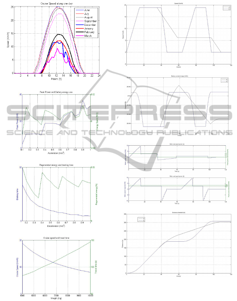
(a) Power delivered by panels and cruise velocity allowed along daytime.

(b) Peak power and battery use vs. acceleration

(d) Cruise speed allowed and travel time vs. weight carried

by the train

Figure 5: Simulation results.

(a) Train speed vs. time.

(b) Battery charge vs. time.

(d) Distance traveled by the train vs. time.

Figure 6: Simulation results for two scenarios: obstacle de-

tection (b) and power cut (a).

the trunk length, braking deceleration, and panel de-

livered power are constant. As expected, the peak

power increases with acceleration. Energy consump-

tion is higher for the highest and lowest acceleration

SIMULTECH2013-3rdInternationalConferenceonSimulationandModelingMethodologies,Technologiesand

Applications

428

(a) Minimum velocity required to reach the target

within schedule.

(b) Battery charge vs. time.

Figure 7: Simulation results for a timed mission.

values. This can be explained since for the highest

values the peak power is higher and therefore more

energy is spent during acceleration. On the other hand

for the lowest values the peak power is lower but it

takes more time for the train to reach cruise speed, so

the acceleration period is longer. Acceleration values

between 0.15 and 0.35 m/s

are often considered as

the range representing a tradeoff between admissible

power peaks, total energy consumption, and passen-

gers comfort. Hereafter, an acceleration of 0.35 m/s

is assumed in all simulations.

Deceleration is also set to a constant value. Brak-

ing time and passengers comfort must also be consid-

ered so the deceleration value should not be too low

nor too high respectively. The corresponding simu-

lation results can be seen in Figure 5c for the energy

regeneration and travel time given a range of possi-

ble deceleration values. Cruise velocity was set to

20 km/h and the track gradient and passenger weight

are considered null. The absolute deceleration value

was linearly increased in order to observe the regener-

ated energy and braking time evolution. As expected,

braking phase duration decreases for higher deceler-

ation values, this happens because the higher the de-

celeration value, the later the train brakes in order to

stop at the station.

Regeneration increases with deceleration. Rea-

sonable values for deceleration are often in the range

-0.6 and -0.8 m/s

. Hereafter, a deceleration of -0.8

m/s

is assumed.

Train weight inﬂuences the power demand and

consequently the velocity of the train. Figure 5d

shows travel time and cruise velocity given the weight

carried by the train, considering the same amount of

power available. It is possible to see that the higher

the weight the lower the cruise velocity reached by

the train. Consequently the travel time increases with

weight. For a weight exceeding 8 tonnes it is possible

to see that the cruise velocity is lower than the mini-

mum value of 10 km/h and the train must use battery

power in order to achieve minimum cruise velocity.

The results of two simulations on different sce-

narios are presented in Figure 6, namely a power loss

that prevents the panels from delivering power (for

instance, cloudy weather), and an obstacle is detected

on the track. The train is intended to travel 1 km and

the power delivered by the panels is 3 kW. The battery

initial charge is set to 7 kWh.

Figure 6a shows the velocity plot for each simula-

tion. For the obstacle scenario the train reaches cruise

speed around time unit 15. At time 40, when the ob-

stacle is detected, the train brakes to full stop. The

obstacle detection is lost at time 65, when the train

accelerates and reaches cruise speed again. Once it

reaches ﬁnal destination it decelerates again until it

stops.

In this scenario it is also possible to see, Figure

6b, that the battery discharges only during accelera-

tion and charges during deceleration, when regenera-

tion occurs. During cruise speed the battery keeps its

charge since the power delivered by the panels is able

to support speed above minimum.

In the ﬁrst scenario once the power loss is de-

tected, the train decelerates until it reaches minimum

speed. This speed guarantees the train reaches the

destination within the time goal. This speed is sup-

ported exclusively by the battery, since the panels are

delivering no power. Figure 6b shows that during this

time the battery is discharging as expected, until the

train approaches the station.

Figure 6c represents the power required by the

motor and the power delivered by the panels. It is

possible to see in Figure 6b that whenever the de-

ViabilityStudyonSupervisoryControlforaSolarPoweredTrain

429

mand is larger than the power delivered, the battery

discharges. This is veriﬁed in the acceleration phase

and also during the power cut, in order to support the

minimum speed.

Figure 6d represents the distance traveled by the

train during simulation. By comparing these graphics

with the speed proﬁle shown in 6a it is possible to see

that the model is consistent.

Accounting for a time schedule was implemented

by feeding the Petri net model with a timing signal

from the external environment. A simulation was

performed where the train is required to travel 1 km

within a maximum time of 360 s. The results are

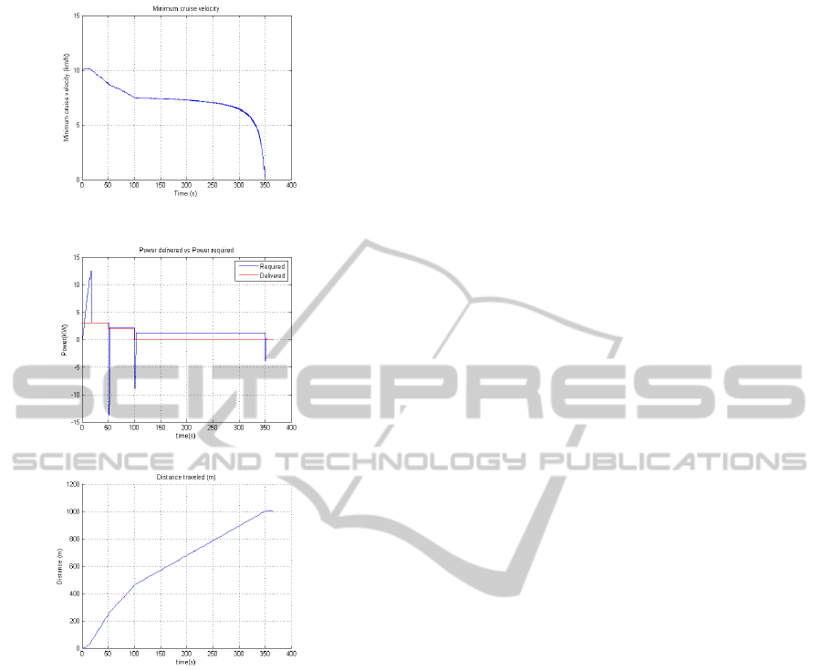
shown in Figure 7.

Figure 7a shows the minimum velocity required

in order to reach the target within the maximum time

given. A higher velocity is allowed as long as the pan-

els are able to sustain it. Through Figure 7b it is pos-

sible to see that until time 100 the panels are able to

sustain a higher velocity, which causes the minimum

velocity value to decrease as time passes. From that

time instant forward the panels stop delivering power,

which causes the train to assume the value of mini-

mum velocity, in order to reach the target in time. The

train travels at this velocity until it stops at the target

within the deﬁned schedule.

7 CONCLUSIONS

This paper describes a simulation tool to assess the

viability of the Helianto solar train project.

The whole infrastructure was modeled as a dis-

crete events system (DES), represented by Petri nets,

and a supervisory controller was designed for the

whole system. Two key toolboxes were used for these

purposes, respectively, QSS and Netlab. The perfor-

mance of the train is analyzed for multiple scenarios

and evaluated based on energy consumption, travel

time and speed achieved.

Simulations are performed on two different sce-

narios. The ﬁrst scenario refers to a situation where an

obstacle is detected on the track and the second refers

to a power cut during travel. Temporal constraints

such as the ones introduced by time schedules are also

accounted for. The results were consistent, showing

that the velocity achieved by the train allowed the mo-

tion to be maintained by the panels alone, resorting to

battery only during acceleration phase, where a power

peak demand occurs, or when a power failure occurs

in order to sustain minimum velocity.

The results obtained show consistency in the sense

that the train behaves as realistically expected and the

energy consumption was effectively managed. More-

over, taking advantage of the ﬂexibility of the Mat-

lab/Simulink environment the overall tool is suitable

for hardware-in-the-loop experiments.

ACKNOWLEDGEMENTS

This work was partially supported by FCT project

PEst-OE/EEI/LA0009/2011.

REFERENCES

State of California Energy Commission and California Pub-

lic Utilities Commission (2013). Go Solar Califor-

nia. http://www.gosolarcalifornia.ca.gov/equipment/

pv modules.php. Accessed January 2013.

Andr

e, J. (2006). Transporte Interurbano em Portugal, vol-

ume 2. IST Press. Lisbon (in Portuguese).

Bogdan, S., Lewis, F., Kovacic, Z., and Meireles Jr, J.

(2006). Manufacturing Systems Control Design: A

Matrix Based Approach. Springer.

Davidrajuh, R. (2008). Developing a New Petri Net Tool

for Simulation of Discrete Event Systems. In Procs.

2nd Asis Int. Conf. on Modeling and Simulation.

G. Cassandras, C. and Lafortune, S. (2008). Introduction to

Discrete Event Systems. Springer.

Godoy Simaes, M., Franceschetti, N., and Adamowski, J.

(1998). Drive System Control and Energy Manage-

ment of a Solar Powered Electric Vehicle. In Procs. of

the 13th Annual Applied Power Electronics Conf. and

Exposition (APEC’98), volume 1.

Helianto (2013). The Helianto Project. Available at http://

helianto.ist.utl.pt.

Jinrui, N., Fengchun, S., and Qinglian, R. (2006). A Study

of Energy management System of Electric Vehicles.

In Procs. IEEE Vehicle Power and Propulsion Conf

(VPPC’06).

Moody, J., Yamalidou, K., Antsaklis, P., and Lemmon, M.

(1994). Feedback control of Petri nets based on place

invariants. Lake Buena Vista.

Netlab (2008). Petri Net Toolbox: Netlab. Available

at http://www.irt.rwth-aachen.de/en/fuer-studierende/

downloads/petri-net-tool-netlab/.

QSS (2008). QSS-Toolbox. Available at http://

www.idsc.ethz.ch/ Downloads/ qss.

SoDa (2012). SoDa, Solar Radiation Data. http://

www.soda-is.com. Accessed January 2012.

SRoeCo Solar (2013). Most Efﬁcient Solar Panels.

http://sroeco.com/solar/most-efﬁcient-solar-panels.

Accessed January 2013.

SIMULTECH2013-3rdInternationalConferenceonSimulationandModelingMethodologies,Technologiesand

Applications

430