Modeling “Info-chemical” Mediated Ecological System by using Multi

Agent System

Yasuhiro Suzuki and Megumi Sakai

Department of Complex Systems Science, Graduate School of Information Science, Nagoya University,

Furocho Chikusa, Nagoya City, Japan

Keywords:

Multi Agent System, Simulation of Ecological Systems, Chemical Ecology, Evolution of Agent Communica-

tion Languages.

Abstract:

We model and simulate an ecological system, where each agent (plants, herbivores and carnivores) commu-

nicate with each other by using communication languages of chemical volatiles (info-chemical signals). This

info-chemical signals are produced by plants when they are suffered from feeding damage of herbivores and

natural enemy (carnivores) of the herbivores are attracted by the signal. In this ecological system, since carni-

vores learn the signal and trace it, plants try to endure the feeding damage until the population of herbivores

become large and enough herbivores can supply for the carnivores, otherwise carnivores are not to be attracted

by the signal and try to explore more valuable signal. However, it has reported that, some mutated plants

produce chemical signals soon even if there are few or no herbivores and attract carnivores (cry wolf plants).

We model the ecological system which cry wolf plants by using the MAS. without geographic space and with

geographic space. And we conﬁrm that in the both types of models, in order to escape from cry wolf plants,

“honest plants” produce different types of signals so various types of signals emerge. Interestingly, in the

system with geographic space, if there is a “colony” of cry wolf plants then signal does not evolve and honest

signal and cry wolf signal can coexist.

1 CHEMICAL ECOLOGY,

ECOLOGICAL SYSTEMS WITH

INFO-CHEMICAL SIGNALS

In the science of (theoretical) Ecology, plants have

been considered as “resources” of the food chain in

the ecological system, where herbivores feed plants

and carnivores feed herbivores. Hence ecological sys-

tems have been described as interactions between her-

bivores and carnivores such as Lotoka-Volterra model

(Lotoka, 1910);

X = aX − bXY, (1)

Y = bXY − cY, (2)

where X is the population of herbivores and Y, carni-

vores.

However in the Chemical Ecology (Dicke and

Takken, 2008), it has turned out that plants are not

just resources but participating in the ecological sys-

tem as “a player”; they cannot run away or remove

herbivores directly but they can indirectly protects

themselves by attracting herbivores’ natural enemy

(carnivores) by producing signals; when plants are

suffered from feeding damage, they produce volatile

chemicals as “SOS signal” and attract natural ene-

mies. Plants are able to produces about twenty kinds

of signals properly and attract appropriate natural en-

emy according to the types of herbivores (Dicke and

Takken, 2008). Carnivores learn the signal and ex-

plore herbivores by tracing the signals. Hence plants

endure the feeding damage until enough herbivores

can supply for the carnivores otherwise carnivores

learn that the signal is not useful and they are not to be

attracted by the signal and explore more valuable sig-

nal (Dicke and Takken, 2008). In contrast, it has been

reported that some mutant plants produces ’cry wolf’

signals; such mutant plants produce large amount of

chemicals when they suffered small feeding damage

by a few herbivores. Such cry wolf plants produce the

same chemical as honest plant producing chemicals

(Shiojiri et al., 2010).

Shiojiri et. al. reported that “the composition

of the herbivore induced volatiles show little change

with the number of herbivores inﬂicting damage to the

plant, but the amounts of volatiles and the responses

of the enemies increase signiﬁcantly. Signal quan-

318

Suzuki Y. and Sakai M..

Modeling “Info-chemical” Mediated Ecological System by using Multi Agent System.

DOI: 10.5220/0004332803180323

In Proceedings of the 5th International Conference on Agents and Artiﬁcial Intelligence (ICAART-2013), pages 318-323

ISBN: 978-989-8565-38-9

 2013 SCITEPRESS (Science and Technology Publications, Lda.)

tity may therefore provide information to the enemies

about herbivore abundance.” so such plant signals is

called ’honest’ signal (Shiojiri et al., 2010).”

In the case when most of the plants emit hon-

est signal, mutant plants (cry wolf plants) can gain

protection from herb-ivory, because visited carnivores

will remove herbivores already present. However the

number of herbivores in the cry wolf signaler are a

few for carnivores they learn such signal is not use-

ful. As (Sabelis et al., 2011) point out, when a honest

signal has been commonly used, cry wolf plants can

take advantages to use the signal and may increase its

population. However, carnivores will learn the signal

as “dis-honest” signal and carnivores may not be at-

tracted by the signal very much. So in order to keep

on attracting carnivores, honest plants haveto produce

“new-and-honest” signals. Some theoretical models

predict that co-evolution of signals will emerge in this

system (Sabelis et al., 2011; Jansen and van Baalen,

2003).

2 METHOD OF MODELING AND

SIMULATION

We model and simulate the ecological system by us-

ing two types of systems; system without / with geo-

logical space. In the system without geological space,

we regard the system as “chemical reactions,” where

each agent is chemical substance and reacts with each

other by reaction rule; such a MAS is called the Artiﬁ-

cial Chemistry (Dittrich et al., 2006). And the system

with geological space is composed of the two dimen-

sional Cellular Automaton.

2.1 Artiﬁcial Chemistry, Abstract

Rewriting System on Multisets,

ARMS

Formally, an Artiﬁcial Chemistry, AC can be deﬁned

by a triple (A, R), where A is the set of molecules, R

is a set of reaction rules representing the interaction

among the molecules (Dittrich et al., 2006). Various

ACs have been proposed and applied in modeling and

simulation of complex systems (Dittrich et al., 2006).

In this study, we use a model of AC, Abstract Rewrit-

ing System on Multisets, ARMS (Suzuki et al., 1996).

ARMS have been used on modeling and simulation of

non-linear chemical reactions (Suzuki et al., 2001),

Systems Biology of the cell (Suzuki et al., 2001), a

model of Origin of Life (Suzuki et al., 2001), Social

Systems and so on.

In ARMS a chemical solution is a ﬁnite multi-

set of elements denoted by symbols from a given al-

phabet, A = {a, b, . . . , }; these elements correspond to

molecules. A reaction rule is a pair of two multisets,

l, r and it rewrites a multiset, mc; if the multiset l is in-

cluded by the multiset then l is removed from the mc

and r is merged with it, so a rewriting is expressed as

mc− l + r, where “+ and -” are addition and deletion

on a multiset.

2.2 How does ARMS Work?

Example. We give R = { a,a,a → c : r

, b → d :

, c → e : r

, d → f, f : r

, f → g : r

}. and assume

that set the initial state as {a, a, b, a}. In this example,

the reaction rules are applied in parallel (the strategy

of applying rules is not only limited in parallel but

also rules can be applied rules in sequential or maxi-

mally parallel). Figure 1 illustrates a sequence of re-

{a, b, a, a} ⊆ a, b

↓ (r

, r

)

{c, d} ⊆ c, d (the left hand side of r

, r

)

↓ (r

, r

)

{e, f, f} ⊆ f (the left hand side of r

)

↓ (r

)

{e, h, h} There are no rules to apply, so it reaches

the halt state

Figure 1: Example of ARMS reaction steps

action steps, For {a, a, b, a}, r

and r

are applied and

it is transformed into {c, d} and r

and r

rewrite it to

{e, f, f }; no rules can rewrite it so rewriting halts.

3 MODEL WITHOUT

GEOGRAPHIC SPACE

It has been reported that every honest plant produces

almost same quantity of HIPV and threshold of the

population of herbivores for start producing HIPV

almost the same (Dicke and Takken, 2008; Shiojiri

et al., 2010). Hence we can estimate the degree by

feeding damage by herbivores based on the quantity

of the HIPVs. So we deﬁne the biomass of plants,

P as P− ΣH

, where H

is the total quantity of every

HIPVs; if the quantity of HIPVs are small, there are

few herbivore and, large quantity of HIPVs indicates

there are many herbivores.

The model is composed of honest signal, h

, dis-

honest signal, c

and a carnivore which is attracted

by h

or w

; where the sufﬁx “i” indicates the type of

chemical proﬁle of HIPV. Plants produce h

and the

carnivore is attracted and remove herbivores. When

Modeling"Info-chemical"MediatedEcologicalSystembyusingMultiAgentSystem

319

the population of honest signal increased, dis-honest

signal of it emerges and if a carnivore is attracted

by the dis-honest signal, it learns the signal is dis-

honest and does not to be attracted by the honest sig-

nal. Hence, if the dis-honest signals increased, hon-

est plant produces different chemical proﬁle of HIPV.

Honest plants can not know, how manydis-honest sig-

nals are produced, however if they can not produce

different type of HIPV and attract carnivores, they

may go extinct. Hence, if the honest plants survive

under the large quantity of dis-honest signals, it indi-

cates that honest plants can produce different type of

HIPV. On the other hand, when the quantity of dis-

honest signals is small, if a honest plant produces dif-

ferent type of HIPV, carnivores may not to be attracted

to the new HIPV, because they do not have to learn it

is dis-honest signal (in fact, it is not dis-honest signal

because of the population of dis-honest signal is low).

Hence when the the quantity of dis-honest signal

is large, if the honest plant using the same chemi-

cal proﬁle as dis-honest signal is mutated and can

produce new honest signal and attract carnivores in-

creases its population, therefore it can be regarded as

if the population of dis-honest signal increases, there

emerges new honest signal. In this model, the proba-

bility of emergence of new HIPV is deﬁned as

Σh

Σ(h

+ w

)

> τ,

where h

indicates the honest signal of type i and w

the dis-honest signal of type i and τ is the threshold

value of emerging the new type of HIPV.

The model is composed of following reaction

rules;

→ h

, h

→ c

, h(r

, h

→ c

→ w

, h

, w

→ w

→ ⊥(r

where r

expresses the population growth of herbi-

vores; as the population of herbivores is increased, the

quantity of HIPV is also increased. r

expresses the

HIPV attracts carnivores and r

expresses attracted

carnivores remove herbivores. r

expresses mutation

of plants from honest to cry wolf plant and r

ex-

presses the learning of carnivores; they learnt and

avoid to be attracted by the HIPV so the population

of carnivores go to the HIPV is decreased. r

and r

are natural death of dis-honest plants and carnivores.

3.1 Result of Simulation

We set the reaction constants, k

to k

as 0.9, 0.5, 0.5,

0.4, 0.5, 0.5, 0.5, respectively, τ = 0.6 and the quantity

of honest signal is 30, the quantity of dis-honest sig-

nals and the number of carnivores are zero, in the ini-

tial state; this parameter setting indicates the growth

of herbivore is high and the mutation rate from honest

plant to wolf is small. Since the quantity of dis-honest

signal is not too large, HIPV does not evolve (Fig-

ure 2). Next, we increase the quantity of dis-honest

Figure 2: When the quantity of dis-honest signals are not

too large, upper line indicates the quantity of honest sig-

nal and below, dis-honest signal; the vertical axis illustrates

the quantity of HIPV (both honest and dis-honest signals)

and the horizontal axis illustrates the steps. The biomass of

plant is 10,000 so the plant biomass reaches to near zero

signals and retarded carnivores attractiveness to the

HIPV, in order to realize it, we change the reaction

constants for the rule of w

, c

→ w

). We set k

to k

as 0.9, 0.5, 0.5, 0.7, 0.5, 0.5, 0.5, respectively,

τ = 0.6 and the quantity of honest signal is 30 and

quantity of dis-honest signals and the number of car-

nivores are zero, in the initial state. In this case, HIPV

evolved and various types of HIPV emerge (Figure 3).

Figure 3: When the quantity of dis-honest signals are large,

each lines indicates the quantity of honest and dis-honest

signals; the horizontal axis illustrates the quantity of HIPV

(both honest and dis-honest signals) and the horizontal axis

illustrates the steps.

ICAART2013-InternationalConferenceonAgentsandArtificialIntelligence

320

4 MODEL WITH GEOGRAPHIC

SPACE

We model the system by using two dimensional Cel-

lular Automaton (2DCA); the geographic space is

square lattice and the eight cells surrounding a cen-

tral cell (Moore neighbour); in the initial state, plants

are distributed on the lattice; every plant grows in the

same growth rate and when the its size (we call the

size of a plant as “biomass” in the below) reaches the

given value, stop growing and a new plant sprout in

the neighbouring empty space.

In several randomly selected plants, herbivores

come and start feeding; they increase the population

by feeding and if the number of herbivoresexceeds its

biomass, the plant goes to die out and all herbivores

move and distribute randomly to the nearest plants;

plants start producing chemical signal when the popu-

lation of herbivores exceeds the given threshold (hon-

est plant). Each carnivores search the chemical signal

by walking on the lattice, carnivores expense “phys-

ical power” by walking and if a carnivore ﬁnds the

plant which has been suffered from feeding damage

by herbivores (we call such a plant as “patch” in

the below) , the carnivore removes all herbivores and

gains its physical power according to the number of

herbivores in the plant, while if a carnivore spends all

physical power before ﬁnding the plant having feed-

ing damage, it goes to die.

4.1 Cry Wolf Plant and Evolution of

Signal

When a new plant sprouts, randomly selected plant

become “cry wolf plant” and it generates chemical

signal when it is suffered from small amount of feed-

ing damage; in the initial state, there are no cry wolf

plants and all plants and carnivores uses the same sig-

nal; however in the lapse of steps, the number of cry

wolf plants increase and carnivores attract to such cry

wolf plants. Each carnivore judges the quality of sig-

nal by “(the number of herbivores in the plant) / (the

distance from the former patch) = Evaluation Value

(EV)”, if the EV is lower than given threshold, the

carnivore judge and learn the plant as cry wolf and

attractiveness of the signal becomes low. Hence as

the population of cry wolf plants increases, the attrac-

tiveness of carnivores becomes low, so honest plants

have to produce different HIPV. In ecological sys-

tems, different HIPVs are continuously generated by

mutated plants (Shiojiri et al., 2010), if there are no

cry wolf plants, carnivores do not learn other HIPV

and plants producing different type HIPV can not at-

tract carnivores and die out, however if the population

of cry wolf plants increases, carnivores explore differ-

ent HIPV randomly so such mutated plants can have

the possibility to attract carnivores.

Learning of a Carnivore

In order to implement learning activity of a carnivore,

we use the simple stochastic model, the polya’s urn;

this model is composed of a urn (pot) and balls, balls

are painted with some sorts of colors. In this model,

history of picking up a ball is remembered through

following way; let us assume that there are three types

(colors, red, black, white) of balls in a pot and the

number of each colored balls are same (for simplicity,

we assume that there are same number of each colored

balls in the urn, here); when a “black” ball is picked

up from the pot, n, (n > 0) black balls are returned to

the urn, hence the probability of selecting a black ball

is increased, compared with other colors. We express

the type of HIPV as the color of ball and the popu-

lation of each HIPV as the number of balls. When

a carnivore judges a HIPV as “honest signal” n balls

of HIPV are added to its memory (urn) and if judges

as “cry wolf”, m balls of HIPV are removed from the

memory and the m balls of “random walk” are added

instead of them; when the carnivore select the ball of

random walk, it explore nearest HIPV randomly.

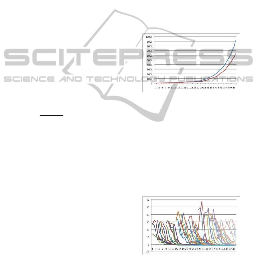
5 RESULT OF SIMULATION

In the model with geological space, when the popu-

lation of cry wolf plants increase, carnivores explore

different type of HIPV and HIPV evolves (Figure.4).

However, as the types of HIPV becomes larger, the

Figure 4: The time evolution of population of HIPV; each

lines illustrates different HIPV.

number of plants producing each HIPV become rela-

tively low; for example when there are 100 plants and

produce two types of HIPV, if 50 plants produce the

same HIPV, the probability of ﬁnding each of HIPV

is 50/100, however if each of plant produces differ-

ent HIPV, the probability of ﬁnding each of HIPV be-

comes 1/100; so as the types of HIPV increase, the

Modeling"Info-chemical"MediatedEcologicalSystembyusingMultiAgentSystem

321

most of carnivores expense all physical power before

ﬁnding out the target HIPV producing plant and they

go extinct. We conﬁrmed this phenomenon in this

model; this phenomenon is called the “Tower of Ba-

bel” and several theoretical contributions have been

addressed it (Jansen and van Baalen, 2003). Hence,

cry wolf plants may induce “Tower of Babel” effect,

but we discover that when they form a “patch” in

the geographic space, HIPV does not evolve and the

Tower of Babel does not emerge (Figure5).

Food Court in an Ecological System

When cry wolf plants are sparsely distributed, carni-

vores may move long distance and meet a cry wolf

plant, it expenses physical power largely but can not

regain the power very much, because there are few

herbivores and it does not enough for long traveled

carnivore; However, if cry wolf plants form a patch,

carnivores do not have to travel long distance and just

hop around cry wolf plants and obtain herbivores;

even if the population of herbivores in each plant is

small, if it is a large patch, it will be able to offer

enough herbivores to carnivores as a whole of the

patch.

And honest plants do not produce HIPV soon, so

carnivores have to wait until population of herbivores

increases, but cry wolf plants produce HIPV soon

and they can offer small amount of herbivores; so to

speak, honest plants serve “full course meal” and cry

wolf plants serve “light meal”; a patch of cry wolf

plants is regarded as a “food court of light meals”

hence carnivores do not judge the HIPV of cry wolf

plants forming a patch as “honest signal” and HIPV

does not evolve (Figure 5). In simulations, we use

the same number of cry wolf plants and compare the

case when they are distributed randomly with placed

gathered; and conﬁrm that in the former case, HIPV

evolves and in the latter case, HIPV does not evolve.

Figure 5: Time evolution of HIPV; each lines illustrates the

different type of HIPV; there are several HIPVs in low con-

centration, they emerges by mutation of plants and changes

of concentration are due to the growth and feeding damage

by herbivores; even if such plant produces HIPV, carnivores

do not learn other HIPV and they can not attract carnivores

and die out

6 DISCUSSION

In order to consider the effect of geographic structure

by using a model without using geographic structure,

we consider a simple example. Let us consider a sim-

ple ARMS: the initial state is {a} and it has a rule

R = {a → a, a}; if we consider this reaction by using

the differential equation,

= a,

this is the Malthus equation and the number of a in-

creases exponentially. However, in this ARMS the

rule is applied sequentially (one rule is applied in the

each step time), the time evolution of computation

which starts from {a} is;

{a} → { a, a} → {a, a, a} → . . . ,

hence the increment of the number of a is described

M(a

) = M(a

) + 1,

where M(a

) denotes the multiplicity of a at step time

of i; and the number of a increases lineally.

If the rule is applied in maximally parallel, the

rule is applied as much as possible in the each step,

the time evolution is {a} → { a, a} → {a, a, a, a} →→

{a, a, a, a, a, a, a, a, a, a, a, a, a, a, a, a} → . . . , so the

increment of the number of a is described as

M(a

) = 2 × M(a

i−1

and the number of a increases exponential (non-

linearly), 2

, (i = 0, 1, 2, ..., ) and time evolution ﬁts

with the Malthus equation.

6.1 Linear, Non-linear and

“Meso”-linear

In the ARMS with the maximally parallel rule appli-

cation, reaction constants are deﬁned for each reac-

tion rule. For example, if we set the reaction con-

stant for the rule a → a, a as 0.5, the expectation value

of applying the rule is 0.5 × the size (cardinality)

of the multiset; so the time evolution is, for exam-

ple {a} → {a, a} → {a, a, a, a} → {a, a, a, a, a, a} →

{a, a, a, a, a, a, a, a, a, }. . ., where the rule is applied in

parallel to bold characters. Hence the time evolution

is neither linear nor non-linear. We namesuch dynam-

ics as “meso”-linear, which means that the dynamics

is in between linear and non-linear. In this example,

when the reaction constant near to 1.0, its behavior

resembles with the Malthus equation and near to 0.0,

resembles linear system.

ICAART2013-InternationalConferenceonAgentsandArtificialIntelligence

322

Figure 6: Simulation of the rate equation of the model of

the Chemical Ecological system in the Section 3; the top is

the same as Differential Eauation and from top to bottom,

non-linearity becomes strong.

6.1.1 System Size and Meso-linearity

If the size of multiset and the reaction constant are

small, the number of applicable rules is to be also

few, on the other hand, if the size of multiset is large,

even if the reaction constant is small, the number of

applicable rules are not so few. In the ARMS with

the rule of a → a, a, the size of multiset in the initial

state is more than 10, each of time evolution is not

so different, however, when the size of multiset is 1

({a}), its time evolution is different from others; we

investigated the time evolution by changing the reac-

tion constants as 1.0, 0.9, 0.8, ..., 0.1 and the size of

multiset in the initial state as 10,000, 1,000, 100, 10,

1 and examine the meso-linearly compared with the

reaction constant is 1.0 (maximally parallel);

We investigate the time evolution of the popula-

tion of a in 10 steps from the initial state, the rule is

applied in maximally parallel with reaction constants

as 1.0, 0.9, 0.8, ... 0.1.

In each step, the difference between the popula-

tion a with the reaction constant is 1.0 and others and

the difference is divided by the size of multiset in the

initial state for normalizing the value; so we conﬁrm

that when the size of multiset is 1, its time evolution is

different from others. We transform the reaction rule

of the model of chemical ecology (r

to r

in the Sec-

tion 3) into the rate equation of chemical reactions and

we conﬁrmed that by inducing meso-linearlity, behav-

ior of time evolutions becomes different (Figure6).

Considering relation between meso-linearity and the

effect of geological space is our future work.

ACKNOWLEDGEMENTS

This work was supported by the JSPS Core-to-

Core Program (No.20004), the MEXT Grant-in-Aid

for Scientiﬁc Research on Innovative Areas (No.

24104002) and Grant-in-Aid for Scientiﬁc Research

(No. 23300317).

REFERENCES

Dicke, M. and Takken, W. (2008). Chemical Ecology.

Springer Verlag.

Dittrich, P., Ziegler, J., and Banzhaf, W. (2006). Artiﬁcial

chemistries - a review. Artiﬁcial Life, 3(7):225–275.

Jansen, V. and van Baalen, M. (2003). Common language

or tower of babel? on the evolutionary dynamics of

signals and their meanings. Proceedings of Biological

Science, 7(270):69–76.

Lotoka, A. J. (1910). Contribution to the theory of periodic

reaction. Journal of Physical Chemistry, 14(3):271–

274.

Sabelis, M. W., Janassen, A., and Takabayashi, J. (2011).

Can plants evolve stable alliances with the enemies’

enemies? Journal of Plant Interactions, 2(2-3):71–

75.

Shiojiri, K., Ozawa, R., Kugimiya, S., Uefune, M.,

Wijk, M., Sabelis, M., and Takabayashi, J. (2010).

Herbivore-speciﬁc, density-dependent induction of

plant volatiles: honest or cry wolf. PLoS One,

17(5(8)):e12161.

Suzuki, Y., Fujiwara, Y., Takabayashi, J., and Tanaka, H.

(2001). Artiﬁcial life application of p systems. In

LNCS, volume 2235, pages 299–346. Springer Verlag.

Suzuki, Y., Tsumoto, S., and Tanaka, H. (1996). Analysis

of cycles in symbolic chemical system based on ab-

stract rewriting system on multisets. In Artiﬁcial Life

V, pages 521–528. MIT Press.

Modeling"Info-chemical"MediatedEcologicalSystembyusingMultiAgentSystem

323