Structural Analysis of Nuclear Magnetic Resonance Spectroscopy

Data

Alejandro Chinea

and José L. González-Mora

Departamento de Física Fundamental, Facultad de Ciencias UNED, Paseo Senda del Rey nº9, 28040, Madrid, Spain

Departamento de Fisiología, Facultad de Medicina ULL, Campus de Ciencias de la Salud, 38071, La Laguna, Spain

Keywords: NMR Spectroscopy, Clinical Diagnosis, Machine Learning Applications.

Abstract: From the clinical diagnosis point of view in vivo nuclear magnetic resonance (NMR) spectroscopy has

proven to be a valuable tool for performing non-invasive quantitative assessments of brain tumour glucose

metabolism. Brain tumours are considered fast-growth tumours because of their high rate of proliferation.

Therefore, there is strong interest from the clinical investigator’s point of view in the development of early

tumour detection techniques. Unfortunately, current diagnosis techniques ignore the dynamic aspects of

these signals. It is largely believed that temporal variations of NMR spectra are simply due to noise or do

not carry enough information to be exploited by any reliable diagnosis procedure. Thus, current diagnosis

procedures are mainly based on empirical observations extracted from single averaged spectra. In this paper,

a machine learning framework for the analysis of NMR spectroscopy signals is introduced. The proposed

framework is characterized by a set of structural parameters that are shown to be very sensitive to metabolic

changes as those exhibited by tumour cells. Furthermore, they are able to cope not only with high-

dimensional characteristics of NMR data but also with the dynamic aspects of these signals.

1 INTRODUCTION

The last decade has seen a rise in the application of

proton NMR spectroscopy techniques,

fundamentally in fields such as biological research

(Raamsdonk et al., 2001) and clinical diagnosis

(Lisboa et al., 2010). The main goal within the

biological research field is to achieve a deep

understanding of metabolic processes that may lead

to advances in many areas including clinical

diagnosis, functional genomics, therapeutics and

toxicology. In addition, metabolic profiles from

proton NMR spectroscopy are inherently complex

and information-rich, thereby having the potential to

provide fundamental insights into the molecular

mechanisms underlying health and disease.

Nevertheless, it is important to note that the main

difficulty is not simply how to extract the

information efficiently and reliably but how to do so

in a way which is interpretable to people with

different technical backgrounds. In fact, machine

learning techniques (Bishop, 1995; 2006) have

recently been recognized by biological researchers

(Ebbels and Cavill, 2009) as an important method

for extracting useful information from empirical

data.

From a clinical diagnosis point of view, proton

NMR spectroscopy has proven to be a valuable tool

which has benefited from the knowledge and

experience acquired through biological research

studies. Furthermore, a large number of proton NMR

spectroscopy applications have targeted the human

brain. Specifically, it has been extensively used for

the study of brain diseases and disorders, including

epilepsy (Aydin et al., 2007), schizophrenia

(Sigmundsson et al., 2003), parkinson's disease

(Summerfield et al., 2002) and bipolar disorder

(Frye et al., 2007) amongst others. This is mainly

due to the fact that proton NMR spectroscopy is a

non-invasive technique, which is particularly

important in this part of the body where clinical

surgery or biopsy is more delicate than in other

areas. In addition, it is important to note that it

allows in vivo quantification of metabolite

concentrations in brain tissue for clinical diagnosis

purposes. Moreover, one of the most successful

applications of proton NMR spectroscopy has been

cancer research (Kwock et al., 2006); (Bottomley,

1984). In this paper, the focus is on proton NMR

brain spectroscopy.

Generally speaking, the process of clinical

diagnosis involves the analysis of spectroscopy

212

Chinea A. and L. González Mora J..

Structural Analysis of Nuclear Magnetic Resonance Spectroscopy Data.

DOI: 10.5220/0004321902120222

In Proceedings of the International Conference on Bioinformatics Models, Methods and Algorithms (BIOINFORMATICS-2013), pages 212-222

ISBN: 978-989-8565-35-8

 2013 SCITEPRESS (Science and Technology Publications, Lda.)

signals obtained from a well-defined cubic volume

of interest (single voxel experiment) in a specific

region of the brain during a pre-defined time frame

(acquisition time). Two acquisition methods are

commonly used, namely point resolved spectroscopy

(PRESS) (Frahm et al., 1987) or stimulated echo

acquisition mode (STEAM) (Nelson and Brown,

1987). Most of the time, the analysis of the signals is

carried out in the frequency domain. The raw signal

from the free induction decays (FIDs) is transformed

using the discrete fourier transform. Afterwards, a

pre-processing stage is also performed to remove

artefacts from the acquisition process. Finally, the

resulting spectral signals, whose number is

approximately equal to the acquisition time divided

by the repetition time of the sequence, are averaged

and in most cases used for a preliminary diagnosis

which relies on a simple visual analysis of the

spectra.

However, current diagnosis techniques based on

proton NMR spectroscopy are still in their infancy.

Firstly, as stated above, powerful tools like machine

learning techniques are scarcely applied within this

context (Sadja, 2006). Indeed, most of the

applications of machine learning techniques have

been in the field of systems biology research

(Friedman, 2004); (Basso et al., 2005) and have used

data from other techniques like liquid

chromatography mass spectrometry or gene

expression microarray. This is mainly due to the

abovementioned problems regarding the

interpretability of the information but also because

of a lack of effective communication of results

between researchers working in different fields. Of

particular interest is the fact that current diagnosis

techniques ignore the dynamic aspects of these

signals. It is largely believed that the information

content of temporal variations of NMR Spectra is

minimal. Thus, current diagnosis procedures are

constrained to empirical observations extracted from

a single averaged spectrum. Furthermore, this fact

could mask important information concerning

metabolic changes, especially in early stages of

tumour formation. In this paper, a machine learning

framework for the analysis of NMR spectroscopy

signals is introduced which is able to exploit both

static and dynamic aspects of these signals.

The rest of this paper is organized as follows: In

the next section, the principal characteristics and

difficulties associated with the processing of H-

NMR signals are presented. In section 3, a formal

characterization of NMR-based data is introduced

from a machine learning point of view. The

reliability of the proposed measures is assessed

through careful analysis of the results provided by a

specific experimental design in section 4. Finally,

section 5 provides a summary of the present study

and some concluding remarks.

2 CHARACTERISTICS OF

H-NMR DATA

The metabolites detectable with proton NMR

spectroscopy include, between others, the

resonances of N-acetylaspartate (NAA), N-acetyl

aspartyl glutamate (NAAG), alanine (Ala), Choline

(Cho), creatine (Cr), gamma-aminobutyric acid

(GABA), glutamine (Gln), and a variety of other

resonances that might not be evident depending on

the type and quality of spectra as well as on the

pathological condition. The molecular structure of a

particular metabolite is reflected by a typical peak

pattern. Furthermore, the area (amplitude) of a peak

is proportional to the number of nuclei that

contribute to it and therefore to the concentration of

the metabolite to which the nuclei belong.

Of particular interest is the fact that even if peak

amplitudes change from different samples reflecting

a change in concentration, the ratios between the

central resonance peak and sub-peaks, composing

the metabolite fingerprint, always remain constant.

Most of the metabolites have multiple resonances

many of which are split into multiplets as a result of

homonuclear proton scalar coupling. Despite high

magnetic fields increase the sensitivity and spectral

dispersion in NMR spectroscopy, at clinical field

strengths (from 1.5 up to 3 Teslas), there exists a

significant overlap of peaks from different

metabolites.

In addition, the response of coupled spins is

strongly affected by the acquisition parameters of

the NMR sequence, e.g. radio frequency pulses

employed and the time intervals set between them

(Cloarec et al., 2005). Furthermore, additional

difficulties are caused by the presence of

uncharacterized resonances from macromolecules or

lipids. This is further complicated by small but

significant sample to sample variations in the

chemical shift position of signals, produced by

effects such as differences in pH and ionic strength.

As a result of this problem, information coming

from a given metabolite contaminates the spectral

dimensions containing information from other

metabolites. In other words, due to this phenomenon

the resonance frequency of certain metabolites can

suffer slight variations from sample to sample.

StructuralAnalysisofNuclearMagneticResonanceSpectroscopyData

213

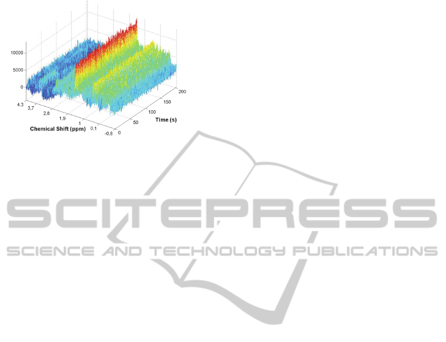
Figure 1: Temporal evolution of the Spectra associated to

a short-TE NMR single voxel brain spectroscopy

experiment at 3T (3 Teslas of Magnetic field strength).

The voxel was located in the visual cortex of a healthy

patient. A total echo time (TE) of 23 ms and a repetition

time (TR) of 1070 ms were used for the acquisition

process conducted during several minutes. The molecular

structure of a particular metabolite is reflected by a typical

peak pattern. The area (amplitude) of a peak (i.e., the

vertical axis of spectra) is proportional to the number of

nuclei that contribute to it and therefore to the

concentration of the metabolite to which the nuclei belong.

The horizontal axes correspond to the chemical shift scale

(ppm) axis (which is representing brain metabolites

resonances) and the time axis (in seconds) respectively.

For instance, the resonance associated to the N-

acetylaspartylglutamate (NAAG), a dipeptide of N

substituted aspartate and glutamate (that is believed to be

involved in excitatory neurotransmission processes) is

located at 2.046 ppm.

In order to address these problems, some

sophisticated strategies have been proposed

(Bruschweiler and Zhang, 2004); (Keun et al.,

2008). However, the common factor to all the

abovementioned techniques is that they completely

ignore the inherent dynamics of NMR spectroscopy

signals. Unfortunately, it is largely believed that

temporal variations of NMR Spectra (see figure 1)

are simply noise or do not carry enough information

to be exploited by any reliable diagnosis procedure.

For example, in a single-voxel MRS experiment, as

a result of the acquisition process, a whole matrix of

data is obtained from the region of interest.

Furthermore, within that matrix two consecutive

rows correspond to signal frames taken with a time

difference equal to the repetition time set for the

acquisition sequence (usually 1035-1070 ms for

short total echo time sequences). Therefore, the

number of rows (signal frames) is approximately

equal to the acquisition time divided by the

repetition time of the sequence. Indeed, there is a

small number of frames that are used for water

referencing (usually eight) which are suppressed

when generating the data matrix. In addition, each

row represents a spectral signal obtained from the

volume of interest after a pre-processing stage which

transforms the raw FID temporal data into the

frequency domain. The frequency domain is usually

preferred over the temporal domain (Vanhamme et

al., 2001) since this enables visual interpretation.

Moreover, in the frequency domain the NMR

signal is represented as a function of resonance

frequency. Additionally, each column represents a

given metabolite or metabolic signal. The number of

columns depends on the particular pre-processing

technique used, but is usually 8192 or 4096

dimensions, depending whether or not a zero filling

procedure is applied to the transformed signal. In

both cases, the associated chemical shift range

corresponds approximately to the interval [-14.8,

24.8] ppm. However, as stated above, the range of

interest usually taken for brain metabolites is

restricted to the interval [-0.8, 4.3 ppm] leading to a

dimensionality reduction with respect to the original

row size. The exact dimension of these vectors

depends on the procedure used for generating the

chemical shift scale. The water peak and the creatine

peak (i.e., one of the 35 known metabolites involved

in brain metabolism) are commonly used for this

purpose. Nevertheless, it is important to note that the

resulting matrix after selecting the appropriate range

is still composed of high-dimensional patterns.

Afterwards, the temporal variations of the spectra

(i.e. the rows of the matrix of data) are averaged in

order to obtain a single vector (single spectrum

signal). In such vectors each dimension represents

the mean value of a particular metabolic signal.

3 STRUCTURAL MEASURES

In the following sub-sections we introduce a set of

measures that have been used within the context of

supervised learning (Haykin, 1999); (Cherkassy and

Mulier, 2007) for the structural characterization of

NMR-based data sets. The principal advantage of

these characterization parameters is not only their

simplicity but also the fact that they do not make any

assumption about the underlying nature of the data.

Therefore, they are appropriate for dealing with both

static and dynamic data sets.

Without a loss of generality let us suppose a data

set

D composed of N patterns belonging to a

space of dimension d. Furthermore, it is assumed

that each sample of the data set belongs to a

categories

w , Ci 1 , the discriminant function

may also be expressed in terms of the following

indicator function

f , where 1)(



1)( uf

and 0)( uf

otherwise. The classifier

performance may also be expressed by the averaged

classification error:









iji

fCpfE

)(

(8)

The best confusion matrix is that corresponding to

the Bayesian classifier (minimal attainable

classification error). It can be deduced that the

confusion matrix cannot be computed using the

Bayesian classifier as it would imply a perfect

knowledge of the statistics of the problem

(conditional probabilities



wp /



and the a priori

probabilities

p ). Therefore, the best confusion

matrix must be in practice approximated. To this

end, the k-nearest neighbour classifier (Bishop,

1995); (Blayo et al., 1995); (Fukunaga, 1990) is

often used because of its powerful probability

density estimation properties. More specifically, a

set of values for k are generated, for instance the

following odd sequence k = 1,3,5,7,9,11.

Afterwards, a leave-one-out cross-validation

procedure (Haykin, 1999); (Fukunaga, 1990) is

performed for the entire dataset for each k from the

selected set of values. Finally, the best confusion

matrix is that obtained for the value of k which

minimizes the performance error defined in

expression (8).

4 EXPERIMENTS

In this section we consider that the FIDs (Free

Induction Decays) have already been Fourier

Transformed to the frequency domain, and the

artefact removal stage carried out. Furthermore, we

suppose the data is arranged into a matrix in which

each row corresponds to a spectral sample, where

two consecutive rows correspond to signal frames

taken with a time difference equal to the repetition

time of the NMR sequence and each column to a

metabolic signal. The metabolic signal corresponds

to the spectral intensity at a particular chemical shift.

In addition, it is important to note that the metabolic

signals (columns in the data matrix) have values that

differ significantly, even by several orders of

magnitude. Additionally, there are correlations

between them (sample dimensions) due to the

spectral overlap caused by the proton homonuclear

scalar coupling. To take into account the differences

in magnitude of metabolic signals, but allowing at

the same time the possibility to exploit the existing

correlations between them, the whitening transform

(Fukunaga, 1990); (Bishop, 1995) was used to

normalize all the data sets used in this section.

4.1 Data Set Description

For experimental purposes two data sets were used

both of them corresponding to short-TE NMR single

voxel brain spectroscopy. Let us denote the first data

set as A, which corresponds to data collected from

11 healthy patients of ages ranging from 25 up to 45,

with a mean of 31.45 years. The data was collected

from different brain regions (see table 1 for details)

and with approximately equal voxel sizes. The

acquisition time was approximately equal to 5

minutes for all patients, using a total echo time (TE)

equal to 23ms and a repetition time (TR) of 1070ms.

Similarly, the second data set (see table 2 for

details) is a small data set used for comparison

purposes in the experimental settings of section 4.2

and it is composed of data also collected at short TE

but with a slightly different parameterization. Let us

denote the second data set as B. For these data, the

total echo time was set to 35ms and the repetition

time to 1500ms and the patients´ ages ranged from

30 up to 45 with a mean of 36 years. In addition, the

data corresponds to three patients, where data matrix

and B

belong to two healthy patients, while data

matrix B

corresponds to a patient that was

diagnosed with a tumour (after a rigorous clinical

diagnosis procedure including biopsy). In particular,

the data matrix corresponding to patient B

represents data obtained exactly from the brain

tumour area.

BIOINFORMATICS2013-InternationalConferenceonBioinformaticsModels,MethodsandAlgorithms

216

Table 1: Data set A. Illustration of the most relevant

characteristics of the dynamic data set used for the first

experimental setting. This data set is composed of NMR

data collected using a total echo time (TE) equal to 23ms

and a repetition time (TR) of 1070ms from 11 healthy

patients. Each data matrix A

(i =1,2,..,11) is composed

approximately of 300 rows and 1068 columns. In other

words, the samples belong to an input space of 1068

dimensions. The notation used for the voxel location in

NMR Spectroscopy is “Left-Right” (L/R) for the “x”

dimension, “Anterior-Posterior” (A/P) for the “y”

dimension and “Inferior-Superior” (I/S) for the “z”

dimension. Voxel dimensions are expressed in

millimetres.

Data Set A

TE = 23ms

TR= 1070ms

Voxel Location Voxel Size

] [L,P,I]=[0.9,6.3,17.2] [20,20,20]

] [L,P,S]=[8.1,27.7,51.5] [29,20,27]

] [L,P,S]=[6.7,9.5,15.1] [20,20,20]

] [L,P,S]=[0.3,6.6,44.9] [20,20,20]

] [L,P,S]=[1.2,18.5,61.6] [20,20,20]

] [R,P,S]=[0.3,14.6,68.8] [20,20,20]

] [L,P,S]=[2.79,25.97,60.9] [20,18,15]

] [R,P,S]=[21.3,92.8,43.2] [20,20,20]

] [L,P,S]=[27.4,25,63.8] [20,20,20]

] [L,P,S]=[23.2,26.1,38.7] [20,20,20]

] [R,P,S]=[4.1,13.3,45.1] [29,20,27]

Table 2: Data set B. Illustration of the most relevant

characteristics of the dynamic data set used for the second

experimental setting. This data set is composed of NMR

data collected from 3 patients using a total echo time (TE)

equal to 35ms and a repetition time (TR) of 1500ms. Each

data matrix B

(i =1,2,3) is composed approximately of

200 rows and 1068 columns. The data matrix B

corresponds to a patient who was diagnosed with a

tumour. The rest of data correspond to healthy patients.

The notation used for voxel location and the units used for

the voxel size are identical to those used in table 1.

Data Set B

TE = 35ms

TR= 1500ms

Voxel Location Voxel Size

] [L,A,S]=[19.4,14.8,96.3] [16.5,17.7,17]

] [R,A,S]=[20.9,35.5,76.2] [20,29.6,20]

] [L,A,S]=[30,16,64.7] [20,20,20]

All the spectral data were generated and pre-

processed using a spectroscopic and processing

software package from GE Medical Systems

(SAGE). This tool comes with a set of built-in

functions (macro reconstruction operations) which

provide different useful processing options of raw

FID data. We used a macro reconstruction operation

which provides internal water referencing, spectral

apodization, zero filling, convolution filtering and

Fourier transform operation on each of the acquired

frames. However, it is important to note that the

convolution filtering and water suppression options

were not selected. The result of this processing step

is a data matrix where each column represents a

temporal series spectrum of a specific metabolic

signal and each row represents a sample or pattern

from the brain region of interest. Each sample

belongs to a space of 1068 dimensions

corresponding to a chemical shift range of [-0.8, 4.3]

ppm. As mentioned in section 2, this interval

corresponds to the range where the main resonances

concerning the 35 known metabolites involved in

brain metabolism are located.

4.2 Experimental Results

The first experiment conducted was designed to

check the variance of the measures corresponding to

different healthy subjects. At this point, it is

important to remember that both data sets described

in the previous section are dynamic. In addition, the

set of parametric measures introduced in section 3.2

were proposed in a supervised learning context. In

this kind of machine learning paradigm knowledge

about the problem is represented by means of input-

output examples, specifically, examples in the form

of vector of attribute values and known classes. This

means that the samples of the data set must be rated

as belonging to a predefined set of categories. In our

case, the categories are defined according to the

number of different subjects that compose the

database. For data set A there are samples coming

from eleven different individuals, therefore

according to the proposed schema we have eleven

different categories for the samples. Moreover,

samples belonging to subject A

are rated as

belonging to the class C

where i = 1,2,…11. At this

point, it is important to highlight the fact that we

have chosen this categorization scheme for two

reasons: firstly, as stated above, in order to check the

performance of the proposed structural parameters

and secondly, because of a lack of data from patients

presenting disorders that could bias the results.

Ideally, for diagnosis purposes we would have used

just two categories for discriminating disease.

Table 3 (see the appendix for details), shows the

results obtained after computing the dispersion for

data set A after the categorization procedure

described above. The first thing to note is that most

of the dispersion values are below one, thereby

indicating a high degree of overlapping between

classes. These results would suggest that the absence

of substantial differences from data collected from

different patients and brain regions is a plausible

indication of the existence of similar metabolic

processes. It is important to emphasize that

StructuralAnalysisofNuclearMagneticResonanceSpectroscopyData

217

metabolic processes associated to tumour cells are

radically different when compared to those of the

original non-transformed cell types.

However, it is important to note that the

dispersion values associated with categories C

and

with respect to the rest of the categories (rows

and columns A

and A

of the data matrix) are

slightly higher when compared with the rest of the

elements of the matrix. Indeed, there are dispersion

values which are close to unity or even slightly

higher than unity. A careful analysis revealed that

this effect was caused by the voxel size. The size of

the voxel for the “x” and “z“ dimensions (see table

1) is slightly bigger for categories C

and C

with

respect to the standard voxel size [20,20,20]. This is

also true for dimensions “y” and “z” on the voxel

associated with class C

. We observed that the effect

is to some extent proportional to the discrepancy

between the actual size and the standard voxel size.

In order to further validate the results obtained with

the dispersion matrix we computed the Fisher

criterion obtaining a value of 0.8504 which

confirmed the expected overlapping between

classes.

In addition, following a similar procedure we

computed the confusion matrix associated with the

eleven categories composing data set A. Table 4 (see

the appendix for details) shows the best confusion

matrix (see section 3.3) obtained by the KNN

classifier following a leave-one-out statistical cross-

validation procedure. It is important to note that the

estimations of conditional probabilities between

classes shown in the table are multiplied by a factor

of 100 to get percentage values. Therefore, it is easy

to deduce that there is no apparent confusion

between categories as most of the values are zero or

close to zero. Nevertheless, samples belonging to

class C

are apparently the most difficult to classify.

Generally speaking, a high degree of overlapping

given by the dispersion does not necessarily mean

significant confusion between the classes from a

classification point of view. This is an indication of

the existence of multi-modal or very elongated

categories.

The second experiment conducted was designed

to check the sensitivity of the structural parameters

introduced in section 3.2 for detecting the existence

of metabolic changes as a result of including data

samples of a patient who was diagnosed with a

tumour. In turn, this experimental setting also

permitted to assess the influence of the parameters

of the PRESS sequences used. To this end, we

merged the two available data sets A and B (see

section 4.1 for details) to create a unique database.

We followed the same categorization scheme

explained before consisting of assigning as many

categories as the number of patients, where data

samples belonging to the same patient were assigned

to the same category.

Let us denote the merged data set as A+B. It is

important to remember that the samples associated

with data set B were collected using a different

parameterization sequence from that used for data

set A. In particular, for data set B the echo time used

was 35ms and the repetition time 1500 ms. The

fisher criterion computed for this data set led to a

value of 0.8262 indicating overlapping between the

defined categories.

Table 5 (see the appendix for details) shows the

results of computing the dispersion matrix for the

data set A+B. The first thing that can be gleaned

from the table is that most of the values are below

one, thereby indicating the existence of overlapping

between classes from the dispersion point of view.

Therefore, from a dispersion point of view there is

not too much difference between data samples

coming from the two different parameterizations,

although this can be considered to some degree a

logical result taking into account that the echo time

of the two sequences are relatively close.

Nevertheless, the samples associated with the class

representing a disorder (i.e., a patient with a tumour)

led to dispersion values much higher than for the rest

of the values found in the table, even taking into

account the voxel size effect. More specifically, they

are very close or bigger than two (see column B

from table 5) indicating a dispersion caused by the

existence of the disease. At this point, it is important

to remember that the dispersion matrix is not

symmetric. From a geometrical point of view,

according to equations (6) and (10) the strong

dispersion presented by the data samples

representing a disorder (i.e., a tumour) with respect

to the rest of samples indicated a reduced distance in

average from these samples to the centroid of their

category (i.e., category B

). In addition, these results

seem to indicate that classes from healthy patients

are well separated from the class indicating a

disease. Although not shown here, this was also

confirmed by the confusion matrix. Specifically,

from a classification point of view there is no

apparent confusion between the category

representing the patient with a tumour and the other

categories.

Finally, despite our previous considerations

concerning the amount of data, in order to deepen

and further complement the previous results, we

conducted an experiment consisting of using the

BIOINFORMATICS2013-InternationalConferenceonBioinformaticsModels,MethodsandAlgorithms

218

entire database A+B but now defining only two

categories C

and C

to indicate “health” and

“disease” respectively. The categorization procedure

is similar to the procedure described above. All the

samples belonging to data matrix B

were rated as

belonging to class C

, while the rest of the samples

were rated as belonging to category C

. The results

of the dispersion matrix and confusion matrix

computation are shown in table 6. From the

inspection of the table we appreciate that there is a

slight confusion for the recognition of category C

(“disease”). Specifically, there is a certain

probability that patterns belonging to the class

“health” may be rated as belonging to the class

“disease”, although this probability is small, and

from a diagnosis point of view an error of this kind

would be less serious when compared to the

opposite case which is apparently inexistent.

To summarize, tumour cells exhibit radical

genetic, biochemical and histological differences

with respect to the original non-transformed cell

types. We have shown that the fact of using the

dynamical aspects of NMR data together with

relatively simple structural measure like dispersion

and Fisher criterion could substantially help the

diagnosis procedure of the clinical investigator.

Indeed, the aforementioned structural measures used

in a non-supervised learning context have proven to

be very sensitive not only to discrepancies on the

specific parameterizations of the NMR measuring

process (i.e., voxel size) but also to intrinsic

anomalies presented by the NMR data as a result of

metabolic changes in the brain tissue studied. At this

point, it is important to remember that current

clinical diagnosis procedures do not make use of the

dynamical aspects of NMR-based data. Indeed, they

use averaged data (i.e, mean value of the data matrix

of tables 1 and 2). Hence, these results would

invalidate the traditional view that disregards the

dynamic aspects of MRS data as being devoid of

information. This methodical reasoning had been

also previously suggested in (Chinea, 2011) where it

was shown the information-richness associated to

the temporal dynamics of NMR metabolic signals as

a result of its chaotic nature.

Moreover, if the tumour size is relatively small

when compared to the voxel size the fact of using

averages could mask the presence of a tumour.

Although further experiments must be carried out,

for instance using a much larger amount of data,

these preliminary results would suggest that the

proposed structural measures for characterization of

spectral data could be used for the development of

non-invasive early tumour detection techniques. In

addition, these results would also provide a starting

point for the application of more sophisticated

machine learning techniques (Kolen and Kremer,

2001); (Schölkopf et al., 1999) to dynamic NMR

spectroscopy data.

5 CONCLUSIONS

In this paper we have investigated the application of

machine learning techniques to characterize

magnetic resonance spectroscopy data. Throughout

this paper we have focused explicitly on the

characterization of dynamic brain MRS data. We

have presented a formal description of the problems

associated with MRS-based data in terms of its

application context in the field of clinical diagnosis

research. We have shown that the fact of using the

dynamical aspects of NMR data together with

relatively simple structural measures (e.g.,

dispersion, Fisher criterion etc) could substantially

help the diagnosis procedure of the clinical

investigator. Indeed, the aforementioned structural

measures have proven to be very sensitive not only

to discrepancies on the specific parameterizations of

the NMR measuring process (e.g., voxel size) but

also to intrinsic anomalies presented by the NMR

data as a result of metabolic changes in the brain

tissue studied.

Summarizing, traditional clinical diagnosis

methods are characterized by working with averaged

data; conversely, this work attempts to identify

properties of the underlying dynamics using simple

structural measures that were shown to be very

sensitive to metabolic changes as those exhibited by

tumour cells. The principal advantage of the

proposed methodology is not only its simplicity but

also its ability to cope with the high-dimensional

characteristics of spectroscopy patterns which

allowed us to extract the relevant information

required for the detection and diagnosis of disease.

Moreover, the framework presented here opens

the possibility not only of having a starting point for

the use of more complex machine learning

techniques but also for the development of reliable

non-invasive diagnosis techniques using relatively

small experimental data sizes. We hope to have

provided sufficient motivation for further studies

and applications as we believe it is a great challenge

to adopt these methods and to apply them in the

clinical research field.

StructuralAnalysisofNuclearMagneticResonanceSpectroscopyData

219

REFERENCES

Aydin K., Ucok A., Cakir S. (2007), Quantitative Proton

MR Spectroscopy Findings in the Corpus Callosum of

Patients with Schizophrenia Suggest Callosal

Disconnection, AJNR American Journal of Radiology,

28, 1968-1974.

Basso K., M A. A., Stolovitzky G., et al. (2005), Reverse

engineering of regulatory networks in human B cells,

Nature Genetics, 37, 382-390.

Bishop C. M. (1995). Neural Networks for Pattern

Recognition, Oxford University Press, Oxford.

Bishop C. M., (2006). Pattern Recognition and Machine

Learning, Springer Science+Business Media, LLC.

Blayo F., Cheneval Y., Guérin-Dugué A., et al. (1995),

Enhanced Learning for Evolutive Neural Architecture,

ESPRIT Basic Research Project Number 6891,

Deliverable R3-B4-P, Task B4 (Benchmarks), pp. 11-

22.

Bruschweiler R., Zhang F. (2004), Covariance nuclear

magnetic resonance spectroscopy, Journal of

Chemical Physics 120, 5253-5261.

Cherkassy V., Mulier F. M. (2007), Learning from Data:

Concepts, Theory and Methods 2nd Edition, Wiley,

New Jersey, pp.92-127.

Chinea A. (2011), Nonlinear Dynamical Analysis of

Magnetic Resonance Spectroscopy Data, Lecture

Notes in Computer Science 6636, 469-482.

Cloarec O., Dumas M. E., Craig A., et al. (2005),

Statistical Total Correlation Spectroscopy: An

Exploratory Approach for Latent Biomarker

Identification from Metabolic 1H NMR Data Sets,

Analytical Chemistry 77, 1282-1289.

Ebbels T. M. D., Cavill R., Bioinformatic methods in

NMR-based metabolic profiling (2009), Progress in

Nuclear Magnetic Resonance Spectroscopy 55, 361-

374.

Frahm J., Hanioke W., Merboldt K. D., Transverse

coherence in rapid FLASH NMR imaging , Journal of

Magnetic Resonance 72 (1987) 307-314.

Friedman N. (2004), Inferring Cellular Networks Using

Probabilistic Graphical Models, Science, 303, 799-

805.

Frye M. A., Watzl J., Banakar S., et al. (2007), Increased

Anterior Cingulate/Medial Prefrontal Cortical

Glutamate and Creatine in Bipolar Depression,

Neuropsychopharmacology 32, 2490-2499.

Fukunaga K. (1990), Statistical Pattern Recognition, 2nd

Edition, Academic Press, San Francisco.

Haykin S. (1999), Neural Networks: A Comprehensive

Foundation, Prentice Hall, New Jersey.

Jansen J. F. A., Backes W. H., Nicolay K., et al. (2006), H

MR Spectroscopy of the Brain: Absolute

Quantification of Metabolites, Radiology 240, 318-

332.

Keun H. C, Athersuch T. J., Beckonert O., et al. (2008),

Heteronuclear 19F−1H Statistical Total Correlation

Spectroscopy as a Tool in Drug Metabolism: Study of

Flucloxacillin Biotransformation, Analytical

Chemistry 80, 1073-1079.

Kolen J. F., Kremer S. C. (Eds.) (2001). A Field Guide to

Dynamical Recurrent Networks. IEEE Press,

Piscataway, New Jersey.

Kwock L., Smith J. K., Castillo M., et al. (2006), Clinical

role of proton magnetic resonance spectroscopy in

oncology: brain, breast, and prostate cancer, Lancet

Oncology 7, 859-868.

Lisboa P. J. G., Vellido A., Tagliaferri R., Napolitano F.,

et al. (2010), Data Mining in Cancer Research, IEEE

Computational Intelligence Magazine, vol. 5, 1 (2010)

14-18.

Nelson S. J., Brown T.R. (1987), A method for automatic

quantification of one-dimensional spectra with low

signal-to-noise ratio, Journal of Magnetic Resonance

75, 229-243.

Raamsdonk L. M., Teusink B., Broadhurst D., et al.

(2001), A functional genomics strategy that uses

metabolome data to reveal the phenotype of silent

mutations, Nature Biotechnology 19(1), 45-50.

Sadja P. (2006), Machine learning for detection and

diagnosis of disease, Annual Review of Biomedical

Engineering 8, 537-565.

Schölkopf B., Burges C. J. C., Smola A.J. (Eds.),

Advances in Kernel Methods—Support Vector

Learning, MIT Press, Cambridge, MA (1999), pp.

327–352.

Sigmundsson T., Maier M., Toone B. K. (2003), Frontal

lobe N-acetylaspartate correlates with

psychopathology in schizophrenia: a proton magnetic

resonance spectroscopy study, Schizophrenia

Research 64, 63-71.

Summerfield C., Gómez-Ansón B., Tolosa E., et al. (2002)

Dementia in Parkinson disease: a proton magnetic

resonance spectroscopy study, Archives of Neurology

59, 1415-1420.

Vanhamme L., Sundin T., Hecke P. V., et al. (2001), MR

spectroscopy quantitation: a review of time-domain

methods, NMR in Biomedicine 14, 233-246.

BIOINFORMATICS2013-InternationalConferenceonBioinformaticsModels,MethodsandAlgorithms

220

APPENDIX

Table 3: Illustration of the dispersion matrix computed for data set A when the categories (i.e., classes in a supervised

learning context) of the data samples are defined according to the number of different subjects that compose the database.

Specifically, samples belonging to subject Ai are rated as belonging to category C

. Dispersion values close to or lower than

one indicates a high degree of overlapping between the involved categories. Conversely, dispersion values bigger than one

provide an indication that these categories are well separated.

0 0.76 0.21 0.24 0.10 0.14 0.30 0.27 0.20 0.27 0.95

0.79 0 0.80 0.67 0.73 0.73 1.12 0.96 0.74 0.77 0.46

0.22 0.80 0 0.29 0.17 0.21 0.28 0.26 0.23 0.30 1.02

0.26 0.68 0.30 0 0.24 0.23 0.46 0.39 0.26 0.27 0.83

0.12 0.77 0.17 0.24 0 0.12 0.25 0.23 0.19 0.24 0.97

0.15 0.72 0.21 0.23 0.12 0 0.31 0.28 0.18 0.21 0.91

0.26 0.92 0.23 0.37 0.20 0.26 0 0.16 0.31 0.33 1.16

0.29 0.96 0.26 0.38 0.22 0.28 0.19 0 0.32 0.34 1.18

0.20 0.71 0.22 0.25 0.17 0.17 0.36 0.31 0 0.21 0.88

0.26 0.71 0.27 0.25 0.21 0.20 0.37 0.31 0.20 0 0.87

0.83 0.38 0.84 0.68 0.76 0.76 1.17 0.98 0.76 0.79 0

Table 4: Best confusion matrix obtained by the KNN classifier computed for the data set A with a Leave One Out statistical

cross-validation method when the categories of the data samples are defined according to the procedure described in table 3.

The values shown in the table corresponding to the estimation of conditional probabilities were multiplied by a factor of

100 to get percentage values. These results show that there is no apparent confusion between the defined categories.

100 0 0 0 0 0 0 0 0 0 0

0 99.45 0 0 0 0 0 0 0 0 0.54

0 0 100 0 0 0 0 0 0 0 0

0.52 0 0 98.94 0 0 0 0 0.52 0 0

8.42 0 0 0.52 91.05 0 0 0 0 0 0

14.73 0.52 0.52 1.05 1.57 79.47 0 0 1.05 1.05 0

0 0 0 0 0 0 100 0 0 0 0

0 0 0 0 0 0 1.57 98.42 0 0 0

0 0 0 0 0 0 0 0 100 0 0

0 0 0 0 0 0 0.52 0 0 99.47 0

0 0 0 0 0 0 0 0 0 0 100

Table 5: Dispersion matrix obtained when merging dynamic data sets A and B, both corresponding to short-TE NMR single

voxel brain spectroscopy. Most of the values are close to or lower to one indicating that categories involved are overlapped.

Nevertheless, the column associated to category B

presents a strong dispersion with respect to the rest of categories. The

sensitivity of the dispersion for this category is due to the fact that data samples corresponding to category B

correspond to

brain tissue that exhibited strong metabolic changes because of the tumour cells.

0 0.75 0.21 0.24 0.10 0.15 0.30 0.27 0.20 0.26 0.93 0.45 2.24 0.20

0.79 0 0.79 0.66 0.72 0.72 1.11 0.96 0.74 0.77 0.46 1.32 3.14 0.88

0.22 0.79 0 0.29 0.17 0.22 0.28 0.27 0.23 0.30 1.00 0.42 2.37 0.23

0.26 0.67 0.30 0 0.23 0.24 0.45 0.39 0.26 0.27 0.82 0.60 2.08 0.29

0.12 0.76 0.18 0.24 0 0.12 0.25 0.23 0.19 0.24 0.95 0.41 2.22 0.18

0.15 0.71 0.21 0.23 0.12 0 0.31 0.28 0.18 0.21 0.89 0.47 2.05 0.21

0.26 0.91 0.23 0.37 0.19 0.26 0 0.16 0.31 0.32 1.14 0.23 2.47 0.23

0.29 0.95 0.26 0.38 0.22 0.28 0.19 0 0.32 0.33 1.16 0.20 2.39 0.26

0.20 0.71 0.22 0.25 0.17 0.17 0.35 0.31 0 0.21 0.86 0.51 2.05 0.28

0.25 0.70 0.27 0.25 0.20 0.20 0.36 0.31 0.20 0 0.86 0.51 1.67 0.29

0.81 0.38 0.83 0.67 0.75 0.76 1.15 0.98 0.75 0.79 0 1.35 2.89 0.93

0.38 1.06 0.33 0.48 0.31 0.38 0.23 0.16 0.42 0.45 1.30 0 2.74 0.34

0.58 0.77 0.58 0.50 0.51 0.51 0.74 0.60 0.53 0.45 0.85 0.84 0 0.62

0.19 0.81 0.21 0.26 0.15 0.20 0.26 0.24 0.27 0.29 1.02 0.38 2.33 0

StructuralAnalysisofNuclearMagneticResonanceSpectroscopyData

221

Table 6: Dispersion and confusion matrixes after merging dynamic data sets A and B and considering only two categories

of samples in the input space: “health” and “disease” respectively. In particular, samples belonging to healthy patients are

rated as belonging to category C

("health") and the rest of samples (i.e., samples belonging to data matrix B

) are rated as

belonging to category C

("disease"). Once again the dispersion is sensitive to the resulting metabolic differences presented

by the brain tissue. From a classification point of view there is no apparent confusion between both categories.

Dispersion

Matrix

0 1.9655

0.1249 0

Confusion

Matrix

95.2721 0

4.7279 100

BIOINFORMATICS2013-InternationalConferenceonBioinformaticsModels,MethodsandAlgorithms

222