Design of Focusing Catadioptric Systems using Differential Geometry

Tobias Strauß

Institute of Measurement and Control Systems, Karlsruhe Institute of Technology (KIT), Karlsruhe, Germany

Keywords:

Optical Design, Meridional Focus, Sagittal Focus, Astigmatism, Fermat’S Principle, Differential Geometry.

Abstract:

In recent years catadioptric systems, consisting of lenses and mirrors, have gained increasing popularity for

the task of environmental perception. However, focusing of such systems is a common problem as it is often

not considered during the design process of the optical system.

This paper presents a novel approach to address focus in the design of optics with rotational symmetry. The

approach does not only adress the construction of catadioptric systems but can also be used to calculate con-

ventional optics. The approach is based on the calculation of the ﬁrst order approximation of meridional and

sagittal focus using differential geometry. Additional conditions like a single-viewpoint can be considered as

well. The derived equations are combined to a set of ordinary differential equations that is used to calculate the

shape of the optical system via numerical integration. The design concept has been veriﬁed by multi-chromatic

ray tracing simulations.

1 INTRODUCTION

In the ﬁeld of computer vision, environmental percep-

tion is an important task. For this, the possibility to

capture a large ﬁeld of view is often desirable. This

can be performed using either ultra-wide-angle lenses

or catadioptric systems consisting of both, lenses and

mirrors (Benosman and Kang, 2001). For the task

of capturing 360

◦

panoramic images catadioptric sys-

tems are more advantageous as their ﬁeld of view can

be inﬂuenced in a wider range.

However, a big problem of today’s catadioptric

systems is their focusing as this is not considered dur-

ing system design. Instead common designs only deal

with the geometric mapping that describes the rela-

tion between image points and corresponding lines of

sight (Hicks and Bajcsy, 2000; St¨urzl and Srinivasan,

2010).

Neglecting wave effects, the light transport

through an optical system can be described using light

rays (Malacara and Malacara, 2003). The geometric

mapping is deﬁned by the principal rays which pass

through the center of the aperture.

To adress focusing we have to deal with beams

of rays. The rays of a single beam can be character-

ized as meridional, sagittal or skew. For systems with

rotational symmetry, the rays that lie in the meridio-

nal plane spanned by the principal ray and the opti-

cal axis are called meridional rays. The sagittal rays

are the rays that propagate in the sagittal plane that

is perpendicular to the meridional plane and contains

the principal ray (see Figure 1). The sagittal plane

changes whenever the principal ray is reﬂected or re-

fracted. Rays that are neither meridional nor sagittal

are called skew.

In general the focus of the meridional rays differs

from that of the sagittal rays and hence not all rays of

a beam focus in one single point. This effect is called

astigmatism (see Figure 2).

Baker and Nayar introduce the problem of defo-

cus blur for catadioptric systems (Baker and Nayar,

1999). Swaminathan uses caustics to describe the fo-

cus (Swaminathan, 2007). However both approaches

only deal with meridional focusing, leaving the sagit-

tal focusing disregarded. Furthermore, the results are

not used in a constructive way to improve the shape

of the optic.

This paper presents an analytical way to calculate

both meridional and sagittal focusing in a ﬁrst order

approximation using differential geometry and Fer-

mat’s principle.

A common approachwhen designing conventionalop-

tical systems is to use an iterative scheme of ray trac-

ing simulations (Glassner, 1989) followed by draft rat-

ing using a so called merit function. In doing so, an

initial system draft can be optimized until a minimum

of the merit function has been found (Smith, 2004).

However, this approach is time-consuming and the

Strauß T..

Design of Focusing Catadioptric Systems using Differential Geometry.

DOI: 10.5220/0004295300840089

In Proceedings of the International Conference on Computer Vision Theory and Applications (VISAPP-2013), pages 84-89

ISBN: 978-989-8565-47-1

 2013 SCITEPRESS (Science and Technology Publications, Lda.)

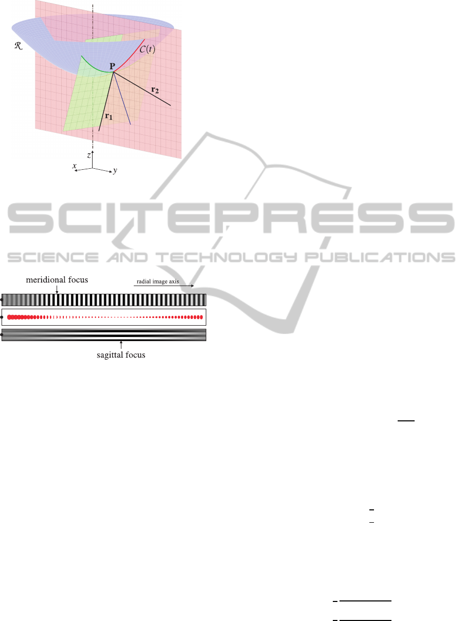
Figure 1: Reﬂection of a principal ray (black) at a surface

of revolution R (blue) obtained by rotating a curve C (t)

around the z-axis. r

and r

denote the direction vector of

the incident and reﬂected ray. The surface’s normal vector

at the intersection point P is colored blue. The red plane is

the meridional plane and one of the sagittal planes is shown

in green. The red and green curve are the corresponding

meridional and sagittal intersection curve respectively.

Figure 2: Simulated defocus blur of a single mirror optic

attached to a conventional lens optic. The black dot in each

sub-image marks the image center. The middle plot shows

spots of several beams of rays along the radial image axis

that can be understood as blur kernels dependent on the po-

sition. Related sample images with vertical and horizontal

stripes visualize the defocus blur. At the meridional focus

point the rays of one beam focus in radial direction, at the

sagittal focus point they focus in circumferential direction.

quality of the optimal draft depends on the number

of parameters used to describe the surfaces.

This paper presents a novel approach to design fo-

cusing optics that directly uses the analytical descrip-

tion of meridional and sagittal focus. In addition, re-

lations for the geometric mapping can be considered -

for example to ensure a single-viewpoint which is es-

sential to be able to remap the image to other projec-

tion models without knowledge about the scene depth.

All equations are combined to a system of ordinary

differential equations describing the shape of the opti-

cal system. This ODE system can be solved quickly

via numerical integration using standard methods like

the Runge-Kutta methods without the need of ray trac-

ing.

2 DESCRIPTION OF FOCUSING

AT BOUNDING SURFACES

The analytical description of focusing at refracting

and reﬂecting surfaces (referred to as bounding sur-

faces) is a central point of this paper. This section

shows how the focusing characteristic of a beam of

rays can be calculated using Fermat’s principle. A

ﬁrst order approximation of a beam’s focusing char-

acteristic is given by its meridional and sagittal fo-

cus point. These focus points describe where rays

focus that propagate within the meridional plane and

sagittal plane respectively. They can be calculated in

closed form using the intersection curve of surface

and corresponding plane (see Figure 1).

2.1 Intersection of Bounding Surface

and Meridional/Sagittal Plane

In the following, we examine a surface of revolution

R which is deﬁned by rotating a curve

C (t) = (0, ρ(t), ζ(t))

(1)

around the z-axis (optical axis). To calculate the fo-

cusing induced by surface R using Fermat’s princi-

ple, we need its intersection curves with meridional

and sagittal plane. Without loss of generality we can

assume x = 0 for the meridional plane. The intersec-

tion point of a principal ray and surface R can be ex-

pressed as P = C (τ). The normalized direction vec-

tors of the incident and refracted principal ray at this

point P are deﬁned as r

= (0, r

, r

)

and r

(0, r

, r

)

respectively. In the following, deriva-

tives with respect to a certain parameter are marked

with this parameter as a subscript, arguments are omit-

ted for the sake of legibility, e.g. ρ

∂ρ(t)

∂t



t=τ

At each intersection point P we can deﬁne the me-

ridional intersection curve and the sagittal intersec-

tion curve. The meridional intersection curve is equiv-

alent to the curve C (t) itself. Its second order Taylor

approximation at P with curve parameter u is given as

M (u) = P+









. (2)

The second order Taylor approximation of the sagittal

intersection curve can be calculated using its mirror

symmetry to the meridional plane and the Taylor se-

ries of C (t) at the intersection point. This yields:

S (u) = P+







(

−r

)

(

−r

)







. (3)

A detailed derivation is omitted due to lack of space.

DesignofFocusingCatadioptricSystemsusingDifferentialGeometry

2.2 Determination of Focus

Given the meridional and sagittal intersection curves,

the corresponding focus points can be calculated us-

ing the laws of geometrical optics. Fermat’s principle

is a compact formulation of these laws which states

that rays of light traverse the path of stationary opti-

cal path length (Hecht, 2001). The optical path length

is deﬁned as the product of geometrical length and re-

fractive index of the surrounding medium.

In a ﬁrst order approximation a beam of meridio-

nal rays neighboring the principal ray focuses in one

point. This point is called the meridional focus point

and lies on the straight line given by the principal ray.

In an equivalent way a beam of sagittal rays focuses

in the sagittal focus point. Thus, given the principal

ray, the focus points can be expressed in terms of their

distances to the surface.

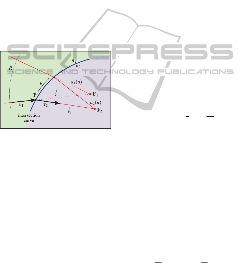
Figure 3: Sketch of the geometric relations used for the ap-

plication of Fermat’s principle. The sketch shows the planar

meridional case. When dealing with sagittal focus, the rays

do not lie within a plane and the problem has to be handled

in 3-dimensional space.

To obtain a description that is also adequate for pa-

rallel rays (intersecting at inﬁnity), we use the inverse

Euclidean distance k between surface and focus point

(see Figure 3). Applying Fermat’s principle the value

of k can be calculated depending on surface curvature

and refractive indices of the adjoining media.

Under the assumption that the incident rays focus

in the virtual focus point F

, they must all have the

same phase (in terms of wave optics) at a circle of ar-

bitrary radius R around F

. Hence it is sufﬁcient to

examine the optical path length between the intersec-

tion with such a circle and the focus point F

. This

optical path length can be written as

w(u) = n

[R− a

(u)] + n

(u) (4)

with the refractive indices n

and n

as well as the geo-

metric distances a

(u) and a

(u).

For the principal ray to pass though point F

, Fer-

mat’s principle says that the corresponding optical

path length must be stationary, so

u=0

= 0. (5)

For the neighboring rays to pass through point F

, ad-

ditionally condition (5) must be satisﬁed in a small

neighborhood which is equivalent to

u=0

= 0 (6)

2.2.1 Meridional Focus

As the meridional focus points F

and F

lie on the

principal ray, their positions can be expressed as

= P+

and F

= P+

(7)

with k

and k

denoting their inverse Euclidean dis-

tance to the intersection point.

Given the local quadratic approximation of the

meridional intersection curve M (u) the optical path

length for the neighboring meridional rays can be

written as

w(u) = n

R− n



M (u) − F



(8)

+ n



M (u) − F



where |.| denotes the Euclidean norm, i.e.:



M (u) − F





−



(9)



−



With (7) the focus points lie on the principal ray. As

the principal ray fulﬁlls the laws of geometric optic

condition (5) is satisﬁed by deﬁnition. To satisfy con-

dition (6) we have to evaluate the second order deriva-

tive of (8) with respect to u at u = 0. After some

longer arithmetic computation this yields:

(ρ

− ζ

)

− (ρ

+ ζ

)

(10)

− n

(ρ

− ζ

)

− (ρ

+ ζ

)

= 0.

This description of meridional focus is equivalent to

the one gained using caustics (Swaminathan, 2007).

2.2.2 Sagittal Focus

As in the meridional case the sagittal focus points F

and F

lie on the principal ray. With the inverse Eu-

clidean distances k

and k

their position can be ex-

pressed as

= P+

and F

= P+

. (11)

VISAPP2013-InternationalConferenceonComputerVisionTheoryandApplications

Given the local quadratic approximation of the sagit-

tal intersection curve S (u), the optical path length for

the neighboring sagittal rays can be expressed equiva-

lent to (8). With the sagittal plane spanned by r

and

condition (6) yields:



ρ(r

− r

)

− k



(12)

− n



+ r

)

ρ(r

− r

)

− k



= 0.

A full derivation is omitted due to lack of space. If we

use the sagittal plane spanned by r

and e

to calculate

the intersection curve and focusing, we get:



+ r

)

ρ(r

− r

)

− k



(13)

− n



ρ(r

− r

)

− k



= 0.

Using the law of geometrical optics, the equations

(12) and (13) can be converted into each other by

some arithmetic computation.

Note that ρ

and ζ

do not inﬂuence the sagittal

focusing directly, but only its change dependent on t.

3 CONSTRUCTION SCHEME

FOR OPTICAL SYSTEMS

The analytical description of the change of focus in-

duced by a bounding surface given by (10) and (12)

will now be used to design optical systems.

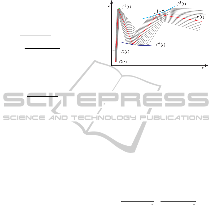
3.1 Parametric Description

In analogy to the last section, systems with rotational

symmetry can be described with a set of planar curves

) with i = 1...N corresponding to N bounding

surfaces. One can choose a parametrization with a

common curve parameter t for all curves C

that is de-

ﬁned in a way that a certain value of t is related to a

certain principal ray (see Figure 4). Such a parame-

terization is the basic step to describe the shape of an

optical system using differential equations.

The parameterization gets unique by the deﬁnition

of the incident principal rays. Here we use two planar

curves O (t) and A (t), where the rays emanate from

O (t) and pass through A (t).

To ensure the validity of parameterization the tan-

gent vectors C

(t) have to be chosen according to

laws of geometrical optics. Each tangent vector de-

pends only on the direction vectors of incident and

reﬂected/refracted ray at the corresponding bounding

Figure 4: A set of planar curves C

(t) can be used to de-

scribe the shape of an optical system with rotational sym-

metry. The curves O (t) and A (t) are used to describe the

incident principal rays. ϕ(t) denotes the exit angle of the

principal rays.

surface. With functions g

(t) and h

(t) dependent on

preceding, current and subsequent intersection point

and scaling functions p

(t) we can write the tangent

vectors C

(t) as

(t) = (0, ρ

, ζ

)

= p

· (0, g

, h

)

. (14)

To determine the meridional intersection curve (2) we

need to know the second order derivative of C

(t) with

respect to t. If we derive (14) w.r.t. t, we get:

(t) =













+ p





. (15)

From a physical point of view, it is obvious that focus-

ing is directly related to the curvature κ

(t). With (14)

and (15) the curvature can be written as:

− ρ









− h

)

+ (h

)

. (16)

So in fact, the curvature is independent on p

and we

can set it to zero in (15). Note that g

and h

are de-

pendent on p

(t), with j ∈ {i− 1,i, i+ 1}.

The scaling function p

(t) is related to the curva-

ture of curve A (t) and hence cannot be chosen freely.

The functions g

and h

are related to the principal

ray’s exit angle ϕ(t) and hence κ

is inﬂuenced by

(t) as well. In summary, we now have a consistent

description of a set of parametrized curves C

(t) with

common parameter t describing the path of the princi-

pal rays and a parameter vector

p(t) = (p

, . .., p

,ϕ

) (17)

that inﬂuences the curvatures κ

at every position t.

DesignofFocusingCatadioptricSystemsusingDifferentialGeometry

3.2 Propagation of Focusing Parameters

With (10) and (12) we are able to calculate the change

of focusing at a single bounding surface. As the para-

meters k

and k

are deﬁned relative to a certain inter-

section point P

they have to be remapped to the next

intersection point P

i+1

before applying these equa-

tions for the next surface. In the following k

denotes

the position of a focus point (meridional or sagittal)

after this remapping. With the Euclidean distance s

between the two reference points the propagation rule

for the focus point description is:

− s. (18)

In order to propagate the change of sagittal focus-

ing dependent on t, which is inﬂuenced by the sur-

faces’ curvatures, we need the ﬁrst order Taylor ap-

proximation of (18). With the linear approximations

k(t) ≈ k

+ k

t and s(t) ≈ s

+ s

t we get:

(t) ≈ k

+ k

t =

1− s

+ s

(1− s

)

t. (19)

In an alternating manner of calculation of focusing

at a bounding surface and propagation of the corre-

sponding parameters to the next surface, we can cal-

culate the object sided focusing parameters k

, k

and

s,t

. As already mentioned, k

cannot be inﬂuenced

directly via the surfaces’ curvatures.

If we want to focus to inﬁnity, we have to satisfy

= 0 and k

s,t

= 0 (20)

and in addition initially ensure that k

= 0.

3.3 Single-viewpoint Condition

Additional conditions can be satisﬁed if the optical

system design has enough degrees of freedom. For

example we can demand a single-viewpoint, which

means that all object sided principal rays intersect in

one point V = (0, 0, v)

on the optical axis. A single-

viewpoint is necessary if we want to remap a captured

image to other projection models like the cylindrical

projection without knowledge of scene depth. In or-

der to satisfy the single-viewpoint condition, the exit

angle ϕ(t) must satisfy

ϕ(t) = arctan



− v



. (21)

So we have to demand

(t) −

− (ζ

− v)ρ

(ρ

)

+ (ζ

− v)

= 0. (22)

3.4 Combined Root Finding Problem

With (20) and (22) we have three root ﬁnding prob-

lems that share a common parameter vector (17). The

task of ﬁnding the corresponding parameter vector

can be formulated as a multi-dimensional nonlinear

least squares problem. To do so, we simply sum

up the squared conditions. Such a nonlinear least

squares problem can be solved using the Levenberg-

Marquardt algorithm. Starting with an initial guess,

this algorithm combines the Gauss-Newton algorithm

with gradient descent to robustly ﬁnd a local mini-

mum. This local minimum should also be the global

minimum with a sum of squared errors equal to zero.

If the value at the local minimum is non-zero the ini-

tial root ﬁnding problem was not solved properly and

we have not found a valid solution.

In general there exists more than one global mini-

mum. A different minimum corresponds to a different

shape of the ﬁnal system and often comes along with

a ﬂipped inside-outside characteristic.

3.5 Final ODE System

The parameter vector (17) and the equations (14) and

(22) deﬁne a set of differential equations for ρ

, ζ

and ϕ (i = 2...N). Given appropriate initial values,

this system of ordinary differential equations can be

solved via numerical integration with standard meth-

ods like the Runge-Kutta methods.

It has to be mentioned that a valid solution can-

not be found for all sets of initial values. Sometimes

it is simply not possible to satisfy the conditions or

the solution’s range of validity is not sufﬁciently large.

However, for appropriate initial values the calculation

of the optical system is very fast.

4 SIMULATION RESULTS

In the last section we presented a construction scheme

for optical systems that directly considers meridional

and sagittal focus as well as a single-viewpoint. This

sections shows ray tracing results for a system draft

that was calculated using this scheme. Ray tracing

was performed using the spline interpolated numeri-

cal ODE solution. Material characteristics leading to

the chromatic dispersion are considered as well.

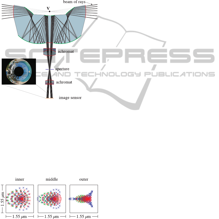
As the construction scheme currently does not

consider chromatic aberration we limited the refract-

ing entry and exit surface in a way that the princi-

pal rays traverse these perpendicularly. To bundle the

beams of rays on the image sensor we use two stan-

dard achromatic lenses (see Figure 5).

VISAPP2013-InternationalConferenceonComputerVisionTheoryandApplications

An additional aperture controls the amount of in-

coming light and higher order defocus blur.

The optical system was calculated for a 1/2.5”

sensor with 8.8 MP. This sensor has a pixel pitch of

1.55 µm. The partially mirrored main lens has a diam-

eter of approximately 55 mm and was calculated to be

manufactured from PMMA. The vertical ﬁeld of view

is approximately 17

◦

Figure 5: Optical design consisting of two standard achro-

matic lenses, an aperture and a mirror lens. The shape of

the partially mirrored main lens was calculated using the

presented design approach. Reﬂecting surfaces are colored

green, refracting surfaces red. The principal ray of each

beam of rays is shown in black, the other corresponding me-

ridional rays are shown in gray color. All incident principal

rays intersect in the single-viewpoint V.

Figure 6 shows the simulated defocus blur and

chromatic aberration at different radial sensor posi-

tions. The spot sizes using an aperture diameter of

1 mm are even below the very small pixel size of

1.55×1.55 µm and let us expect a sharp image.

Figure 6: Simulated defocus blur of inner, middle and outer

beams of rays relating to the image radius. Raytracing

was performed for wavelengths of 500 nm (blue), 550 nm

(green) and 650 nm (red). The colored crosses in each sub-

plot show the sensor positions of different rays emanating

from single object points at inﬁnity.

5 SUMMARY

AND CONCLUSIONS

In this paper we presented a novel approach to de-

sign focusing optics based on differential geometry.

For this, an analytical description of meridional and

sagittal focusing was derived using Fermat’s princi-

ple. The approach considers focusing as well as ge-

ometric constraints. These are combined to a multi-

dimensional root ﬁnding problem, whose solution is

found using the Levenberg-Marquardt algorithm. In

an iterative manner of solving the root ﬁnding prob-

lem and numerical integration the shape of the optical

system is calculated.

A big advantage of this design approach compared

to common approaches based on numerical parameter

optimization is that the shape of the bounding surfaces

is not restricted by a ﬁxed number of parameters used

to describe them.

An exemplary optical draft was analyzed by

means of a multi-chromatic ray tracing simulation.

Future research will focus on the consideration

of chromatic effects arising from refracting surfaces.

This would overcome the limitation that refracting

surfaces have to be traversed perpendicularly to avoid

chromatic aberration.

ACKNOWLEDGEMENTS

The author would like to thank the Hans L. Merkle

Foundation for funding this work.

REFERENCES

Baker, S. and Nayar, S. K. (1999). A theory of single-

viewpoint catadioptric image formation. International

Journal of Computer Vision, Vol. 35.

Benosman, R. and Kang, S. B. (2001). Panoramic Vision:

Sensors, Theory, and Applications. Springer.

Glassner, A. S., editor (1989). An Introduction to Ray Trac-

ing. Academic Press.

Hecht, E. (2001). Optics. Addison Wesley.

Hicks, R. A. and Bajcsy, R. (2000). Catadioptric sensors

that approximate wide-angle perspective projections.

OMNIVIS 2000.

Malacara, D. and Malacara, Z. (2003). Handbook of Optical

Design. Marcel Dekker.

Smith, W. J. (2004). Modern Lens Design. McGraw Hill.

St¨urzl, W. and Srinivasan, M. (2010). Omnidirectional

imaging system with constant elevational gain and sin-

gle viewpoint. OMNIVIS 2010.

Swaminathan, R. (2007). Focus in catadioptric imaging sys-

tems. ICCV 2007.

DesignofFocusingCatadioptricSystemsusingDifferentialGeometry