
On Line-based Homographies in Urban Environments
Nils Hering
1
, Lutz Priese
1
and Frank Schmitt
2
1
Institute of Computational Visualistics, University of Koblenz Landau, Universit¨atsstraße 1, Koblenz, Germany
2
TOMRA Sorting GmbH, Otto-Hahn-Str. 6, M¨ulheim-K¨arlich, Germany
Keywords:
Building Contours, Line Homography, Registration.
Abstract:
This paper contributes to matching and registration in urban environments. We develop a new method to
extract only those line segments that belong to contours of buildings. This method includes vanishing point
detection, removal of wild structures, sky and roof detection. A registration of two building facades is achieved
by computing a line-based homography between both. The known crucial instability of line homography is
overcome with a line-panning and iteration technique. This homography approach is also able to separate
single facades in a building.
1 INTRODUCTION
The location and identification of buildings from 2D
images is a task under much research. There are many
applications, e.g. in Google Street View and similar
concepts of other companies. A combination of GPS
and a compass in a cellular phone can give you rough
information on the landmarks in front of you. The ap-
proach of pose (position and direction) estimation by
matching markers is also well known. We will con-
tribute here to an approach to markerlessly match and
identify a building by its contours.
1
We start with two
images I
1
, I
2
of the same urban environment from dif-
ferent points of view. To match both images we have
two problems:
• Firstly to detect contours of buildings. We present
a rather refined technique to locate and identify the
line segments that solely belong to buildings. This
implies to suppress even strong straight contours not
coming from buildings, even if they intersect orthog-
onally. We will call the resulting set of contours a
“blueprint”, simply because of its visual similarity to
a buildings blueprint.
• Secondly to compute a homography between a
building b in I
1
and I
2
. Point features, such as SIFT or
Harris corners, e.g., are usually quite similar at differ-
ent locations of b and thus cannot be easily used for
corresponding pairs of points in I
1
and I
2
to calculate
a homography. The same holds for the endpoints of
corresponding line segments: usually line segments
1
This work was supported by the DFG under grant
PR161/12-2 and PA599/7-2
of the same line end in two different images in dif-
ferent visible or detectable endpoints. Therefore, we
use corresponding straight lines in a line-based ho-
mography. It is known that a line-based calculation of
a homography is highly unstable. We present a new
algorithm lineHomography to overcome this instabil-
ity that operates with an iterated panning and iteration
technique.
We approach the task to match buildings from im-
age I
1
and I
2
by the following process:
1. Blueprint reconstruction
2. Detection of initial line segment correspondences
3. Initial homography estimation
4. Homography refinement
5. Isolation of single facades
6. Decision: building (facade) matched or not
In this paper we examine the steps 1,3,4,5, and
6. We omit the second step and assume the initial
correspondences to be known. Several methods for
the creation of initial line segment correspondences
are known in literature like (Guerrero and Sags, 2003)
and (Bay et al., 2005), see section 2.
2 PREVIOUS WORK
The analysis of aerial images of urban environments
is widely studied, see, e.g. (Mayer, 1999) and (Balt-
savias, 2004) for an overview. However, detection,
analysis and identification of buildingsin groundlevel
358
Hering N., Priese L. and Schmitt F..
On Line-based Homographies in Urban Environments.
DOI: 10.5220/0004293603580369
In Proceedings of the International Conference on Computer Vision Theory and Applications (VISAPP-2013), pages 358-369
ISBN: 978-989-8565-47-1
Copyright
c
2013 SCITEPRESS (Science and Technology Publications, Lda.)
images has been studied much less and is only re-
cently gaining more and more attention with the ad-
vent of cameras in mobile computing devices like
smartphones and the global availability of ground
level images from services like Google Street View.
A general approach for detection of man-madeob-
jects in images has been introduced in (Kumar and
Hebert, 2003). The algorithm is based on a causal
multiscale random field where the distribution of mul-
tiscale feature vectors is modeled as a mixture of
Gaussians and a set of features typical for man-made
structures is presented. However, this approach seems
more suitable for natural scenes than for urban envi-
ronments.
In (Iqbal and Aggarwall, 1999) an algorithm
which detects whether an image contains a building or
not is presented. For this, the authors search for typ-
ical line junctions in the image. However, they don’t
detect the location of the buildings in the images.
Our approach is inspired by the works of David
(David, 2008) who searches for clusters of lines with
consistent orientation. However, he uses a less in-
volved algorithm for edge extraction and orientation
analysis.
For facade identification an algorithm is presented
in (Zhang and Koˇseck´a, 2007), where the currently
analyzed facade is matched against a set of known fa-
cade images. First a rough preselection is done by
matching color histograms of the facades, whereby
simple 1D hue value histograms are used. Afterwards,
the best matching reference facade is found by the
comparison of SIFT-features (Lowe, 2003).
In (Schmid and Zisserman, 1997) the authors in-
troduce a method which matches line segments be-
tween images by the usage of the known F-matrix.
The aim of this method is to create a basis for the 3D
reconstruction of scenes containing planar surfaces.
In (Guerrero and Sags, 2003) the authors present
a technique for simultaneous line matching and ho-
mography estimation. They start with matching lines
from one image to their nearest neighbor in another
image using a brightness and a geometric criterion.
These first matching candidates are used to compute
a homography which is in turn used to reject wrong
matches and to gain new matches. They use their
method mainly for robot homing. In a continuative
work (L´opez-Nicol´as et al., 2005) a method to com-
pute the motion between two views without know-
ing 3D structure is presented. In this work the basic
matching entities have changed from lines to points.
In (Bay et al., 2005) a method for matching line
segments is introduced. Their scope are uncalibrated
wide-baseline images. They first find matching can-
didates by a color histogram based assginment which
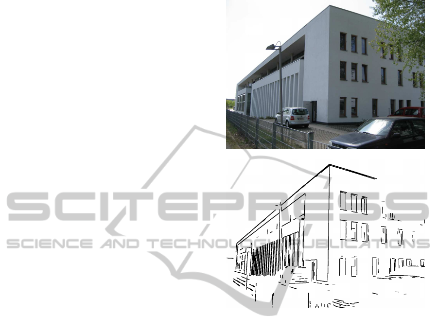
Figure 1: Pair of original and processed image.
is improved by a topological filter. Afterwards ho-
mographies are computed on the base of the initial
matches to gain more matches and to estimate the
epipolar geometry.
An extension of the DLT-algorithm (see (Hart-
ley and Zisserman, 2004)) by lines is presented
in (Dubrofsky and Woodham, 2008). The authors
use both point and line correspondences in this
point-centric-normalized DLT to match images from
hockey videos to a hockey rink model.
3 BLUEPRINT
RECONSTRUCTION
To clearly understand a blueprint reconstruction we
start with the results first. The pair of images in figure
1 present in color a 2D image from an architectural
environment ( the original image). Below of the orig-
inal image the result of our contour extraction algo-
rithm is presented (the blueprint image).
In the blueprint image the essential parts of the
building contours are clearly visible while almost all
OnLine-basedHomographiesinUrbanEnvironments
359
other contoursare suppressed. If one has some knowl-
edge on the geometry of the buildings - say, there oc-
cur only angles of 90 between adjacent straight lines
- even a partial 3D reconstruction from the blueprint
images should become possible.
A freshman in computer vision may ask, where is
the difficulty? Use some straight line detector and the
processing is mainly done. Such straight line detec-
tors are known for decades. They usually transform
the image into grayscale, apply a Canny edge detec-
tor and a Hough transformation. Finally, match the
lines from the Hough transformation with the origi-
nal image to get the contours. However, every expert
who has some experience with straight lines knows
that this will lead to much poorer results, not even
close to the quality in our examples shown e.g. in fig-
ure 1. In principle we follow the mentioned approach
but have to add a whole series of new techniques that
we present now.
3.1 Extraction of Edge Points
and Straight Lines
We regard an image I as a mapping I : Loc
I
→ Val
I
and a pixel P ∈ I as a pair P = (p, v) of a position
in Loc
I
and a value in Val
I
. Of course, Loc
I
is usu-
ally a 2-dimensional and Val
I
a 1- (gray values) or
3-dimensional (color values) array of integers. val(p)
is the value of the pixel at position p.
3.1.1 Extraction of Edge Points
In the first step of our processing chain, we strive to
extract prominent edge points from the image. For
this we use the classic Canny edge detector (Canny,
1986). The result of the canny detector is a set of
straight and curved lines in the image corresponding
to edges. This set can be used to generate a binary
image I
e
of all edges as shown in figure 2.
3.1.2 Straight Line Detection
For a straight line detection one usually applies a
Hough transform on the edges detected by the Canny
algorithm. A Hough transformation of I is a function
h
I
: A → N. A is called the accumulator, an element
b ∈ A a bin. Usually A is of some higher dimension
and a bin is a formal description of an object or a set
of objects in I. h
I
(b) counts how often the object de-
scribed by b appears in the image I. A straight line is
represented in the Hesse normal form and the origin
(0, 0) of R
2
is thought to be in the middle of Loc
I
.
The Hesse normal form describes a straight line l by
two parameters: α, the angle between the normal of
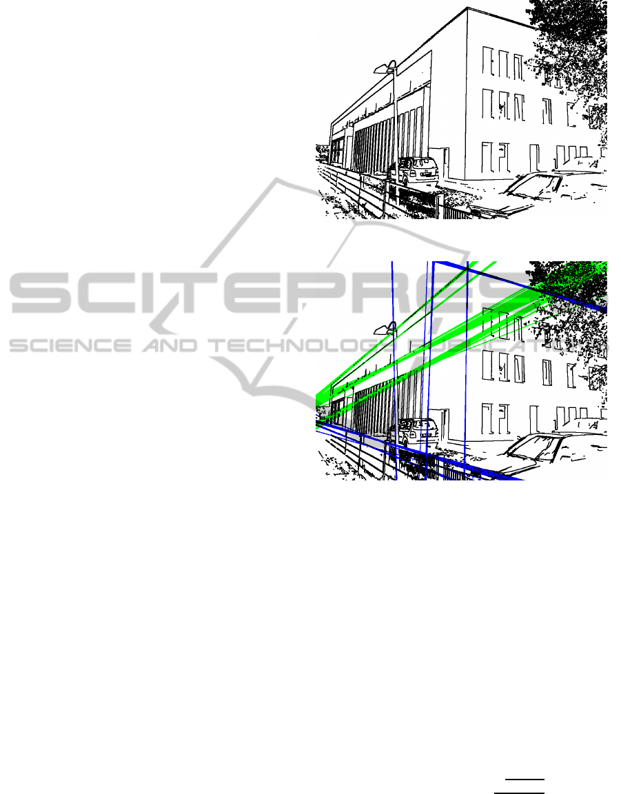
Figure 2: Result of Canny edge detector.
Figure 3: Result of unsophisticated Hough transformation.
the line and the x-axis, and d, the distance between
line and image origin. Thus, the accumulator A is 2-
dimensional with one coordinate for α and the other
for d.
Figure 3 shows the 120 strongest lines found by
an unsophisticated Hough transformation in the canny
output of figure 2. Clearly, such a result is not suffi-
cient for further analysis.
3.1.3 Thinning
We firstly thin out straight lines closely neighbored in
the accumulator. If na is the number of angles and nd
the number of distances representable with the cho-
sen accumulator we apply a non-maxima-suppression
with a square window of width
√
na
2
+nd
2
100
+ 1. Thin-
ning clearly improves results, however it is not suffi-
cient as frequently many prominent lines in the image
are not detected and too often a single line in the orig-
inal becomes a bundle of lines in the transformation.
VISAPP2013-InternationalConferenceonComputerVisionTheoryandApplications
360
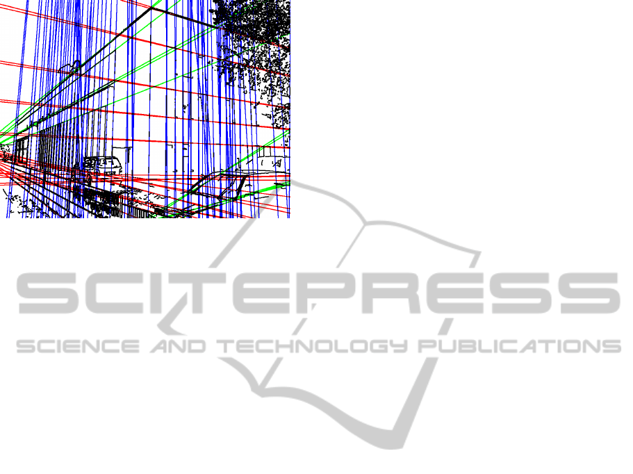
Figure 4: Result of Hough transformation with thinning and
butterfly filtering.
3.1.4 Butterfly Filtering
A second filter from (Leavers and Boyce, 1987)
removes accumulator maxima resulting from edge
points which are not part of longer lines in the im-
age (in outdoor images, such edge points typically oc-
cur, e.g., in trees) by increasing accumulator values in
the middle of the typical butterfly formed structures
resulting from true lines while lessening other accu-
mulator values. When no such filter is applied, the
numerous edges in strongly textured structures often
yield artificial straight lines in the Hough transforma-
tion. Figure 4 shows the best 120 lines after thin-
ning and butterfly filtering. All prominent lines are
detected successfully.
3.1.5 Removal of Wild Structures
Heavily textured areas tend to produce “false” lines
in the Hough transformation, even if a thinning and
butterfly filter is applied. To avoid this, we have de-
veloped in our group a “wilderness map” which char-
acterizes these parts of an image and masks them.
Our algorithm calculates for each pixel a binary
measure classifying the pixel either as wild or non-
wild using binary morphology on the edge image
from the Canny edge detector I
e
. We apply binary
closing with a circular structuring element of radius
4 on I
e
to get the image I
e
′
. In I
e
′
all gaps of a width
of less than 4 pixels are closed. Afterwards an ero-
sion with a circular structuring element of radius 1
is applied on I
e
′
which removes all outer edge points
from I
e
′
. Finally we remove all foreground (e.g. edge)
pixels from I
e
which are also foreground in I
e
′
. The
radius 4 for the closing operation is suitable for our
application scenario of urban environments with im-
ages of size 1024×768 pixels but might have to be
adapted otherwise.
After wild structures are thus removed from the
Canny result I
e
, a Hough transformation is applied.
Figure 5 shows the effect of wilderness removal on
I
e
, figure 6 the effect on the Hough transform. Many
false lines resulting from random Moire structures
(e.g., in the window shutters) are successfully sup-
pressed. Let I
l
denote the binary image of all lines
detected by those combined techniques.
3.2 Vanishing Point Detection
Our improved Hough transform reliably detects the
most prominent straight lines in the image. How-
ever, it remains to choose from these lines those which
are actually part of the favored structures. As we are
mainly searching for structures planar in 3D all paral-
lel lines in those structures will point towards a com-
mon point, the vanishing point. In images showing
architectural environments there are typically two or
three vanishing points corresponding to lines point-
ing upwards, left, and right. We use the vanish-
ing point detector introduced in (Schmitt and Priese,
2009a). This new detector uses several ideas from lit-
erature and combines them with a new intersection
point neighborhood.
The size of this neighborhood depends on the
number of possible intersections of measurable lines,
and, thus, depends on the way one actually computes
the straight lines.
A canonical next step is a cluster analysis of the
measured intersection points. Unfortunately, the in-
tersection neighborhood defines no topology in the
mathematical sense and a cluster analysis technique
without a concept of a distance is required. For this an
adaption of the AGS algorithm introduced in (Priese
et al., 2009) is used that computes an intersection rate
of two sets as a substitute for their distance.
Finally, geometric considerations on the candi-
dates generated by the cluster analysis give the final
vanishing points. Those detected lines pointing to a
vanishing point are further candidates for contours of
buildings.
3.3 Back Projecting into the Image
3.3.1 Straightforward Approach
The lines in I
l
are without endpoints. To get the con-
tours of the desired structures one may match those
lines in I
l
that point to one of the detected vanishing
points with lines segments in the original image, say,
with the edge points generated by the Canny detector.
Let I
vl
be the resulting binary image of all lines point-
ing to a vanishing point in their correct length, i.e.,
OnLine-basedHomographiesinUrbanEnvironments
361
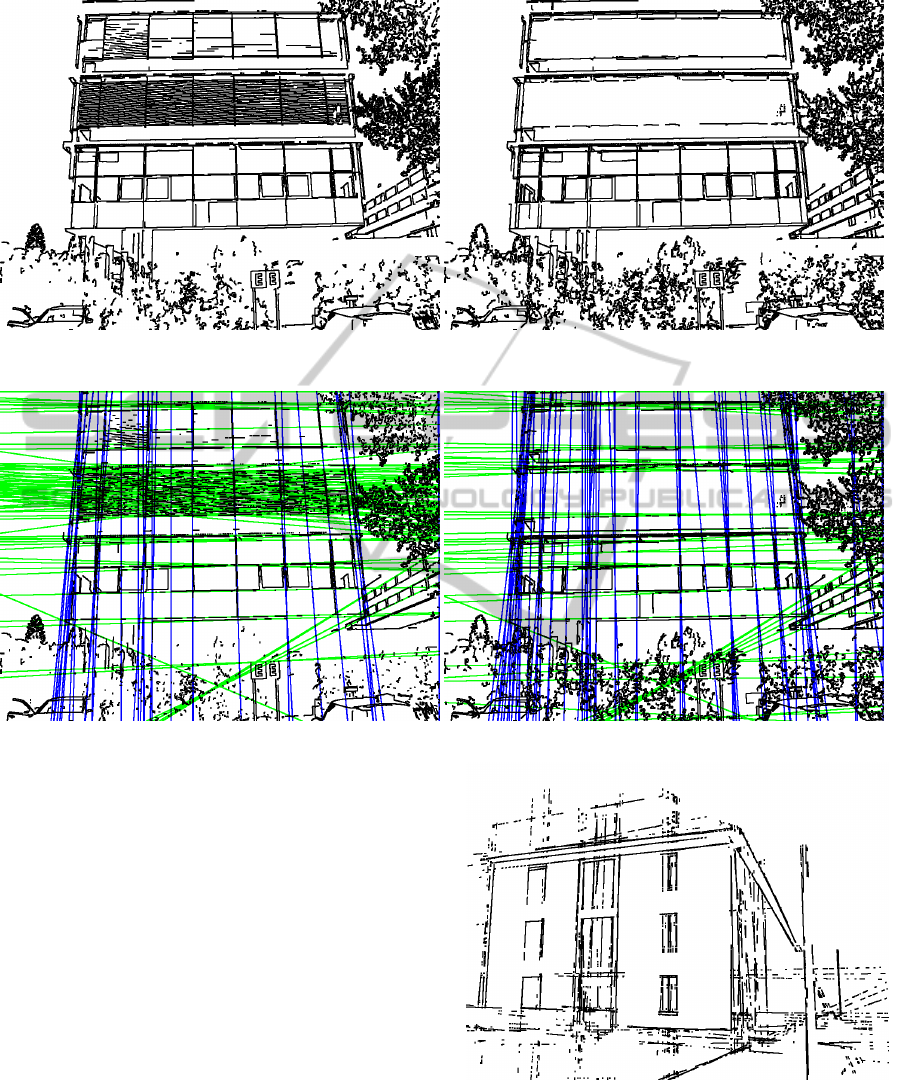
Figure 5: Result of Canny edge detector and result after removal of wild structures.
Figure 6: Result of Hough transformation on normal edge image and result after removal of wild structures.
with endpoints. Figure7 presents I
vl
of an example.
At a first glimpse the results look promising, but there
are two problems.
1. Often the roofs of buildings are not parallel to the
main directions of the building and, thus, do not
point to any detected vanishing point.
2. Not all edges that are part of a contour of a build-
ing appear in a straight line in the Hough trans-
form at all. E.g. window frames often do not con-
tain enough edge points to generate a Hough line.
We therefore do not follow this route.
3.3.2 Refined Approach
To solve problem 1 we compute roof line segments
with a very different method. We firstly apply the sky
detector introduced in (Schmitt and Priese, 2009b).
This sky detector finds the sky rather reliably, no mat-
ter whether the sky is cloudless, partially clouded
Figure 7: Insufficient result after simple back projection of
Hough lines into Canny image.
or overclouded, and works in short as follows. I
is enhanced by a Kuwahara filter (M. Kuwahara, K.
Hachimura, S. Eiho, and M. Kinoshita, 1976) that
smoothens in rather homogeneous regions and simul-
VISAPP2013-InternationalConferenceonComputerVisionTheoryandApplications
362

taneously sharpens edges. After this a CSC seg-
mentation (Priese and Rehrmann, 1993) is applied.
The CSC divides those parts of the sky where the
color is smoothly changing into regions with irreg-
ular bounds. However, parts of a building touching
the sky are segmented into regions with a very regu-
lar boundary towards sky segments, even if the color
of the building is similar to the sky. This distinction
between regular and irregular bounds allows to find a
rather stable sky line. Therefore, this technique would
not work with a split-and-merge segmentation tech-
nique (Horowitz and Pavlidis, 1976). Roof lines are
now found by simply looking for straight parts of the
sky line.
To solve problem 2 we do not combine the de-
tected vanishing points with the results from the
Hough transformation but directly with the Canny im-
age. Note, this doesn’t imply that Hough is not re-
quired as a Hough transformation is essential for the
vanishing point detection. However, after knowing
the vanishing points the Hough lines are no longer
needed. The Canny image I
C
: Loc
I
→ R
2
gives for
any location a gradient strength and gradient direction
(of the detected edge), where too weak edge points
are suppressed and small gaps in longer edges are
closed. The tangent at an image position p ∈ Loc
I
is
the straight through p with direction orthogonal to the
gradient direction at p. A C-line in I
C
is a connected
line in the Canny image, not necessarily straight. We
now process all C-lines in the following way:
• Remove all C-lines with a length of less then 10
pixels.
• Split all C-lines s into sub-C-lines s
1
, .., s
n
such
that for each sub-C-line s
i
there holds:
– the length of s
i
is at least 10,
– the tangents at all pixels in s
i
pass one vanishing
point in a close distance.
The generated sub-C-lines and the roof lines to-
gether form a first blueprint.
3.4 Enhancement
We now enhance this first version of the blueprint and
erase all rather short line segments that are parallel to
a close-by longer line segment. Then we close gaps
between line segment partners. Two lines segments
l
1
, l
2
are partners if one endpoint of l
1
and one of l
2
are in close proximity and l
1
and l
2
point in the same
direction.
4 HOMOGRAPHY BASICS
The following chapter shall give a short summary of
the homography estimation. Especially the line based
homography shall be introduced. Dubrowsky et al.
describe the line-based homography estimation more
precisely in (Dubrofsky and Woodham, 2008). P
2
de-
notes the projective plane. A homography is a linear
invertible mapping h : P
2
→ P
2
where the following
holds: three points p
1
,p
2
and p
3
lie on one line if and
only if h(p
1
),h(p
2
) and h(p
3
) lie on one line.
The general problem is to find a homography h
which maps points p
i
∈ R , 1 ≤i ≤ N, from a plane π
in image I to their corresponding points p
′
i
∈ R , 1 ≤
i ≤ N, on the plane π
′
in image I
′
. The correspon-
dences (p
i
, p
′
i
) are known and the homography h that
satisfies p
′
i
= Hp
i
for all correspondences is in de-
mand.
4.1 The DLT Algorithm
Let p = (x, y) be a point in a two-dimensional im-
age. This point p may be represented as a three-
dimensional vector p
v
= (a
1
, a
2
, a
3
) with x =
a
1
a
3
, y =
a
2
a
3
and a
3
6= 0. The vector p
v
is called a homogenous
representation of p and lies on the projective plane
P
2
.
To compute the projective transformation, the ho-
mography matrix H has to be found. H can be
changed by a multiplication with a constant c 6= 0
without changing the transformation. Hence, H is a
homogenous matrix and has eight degrees of freedom
while it has nine elements. Thus to find H eight un-
knowns have to be determined. We usually identify a
homography h and its matrix H.
The Direct Linear Transform algorithm is an al-
gorithm for the determination of homographies. p
′
i
=
Hp
i
can also be written as c
u
v
1
= H
x
y
1
with c 6= 0
and
H =
h
11
h
12
h
13
h
21
h
22
h
23
h
31
h
32
h
33
!
.
With division of line one by line three and line two
by line three one gets the following two equations:
−h
11
x−h
12
y−h
13
+ (h
31
x+ h
32
y+ h
33
)u = 0
−h
21
x−h
22
y−h
23
+ (h
31
x+ h
32
y+ h
33
)v = 0
One can shape this into Ah = 0 with
A =
−x −y −1 0 0 0 ux uy u
0 0 0 −x −y −1 vx vy v
OnLine-basedHomographiesinUrbanEnvironments
363

and
h = (h
11
h
12
h
13
h
21
h
22
h
23
h
31
h
32
h
33
)
T
.
To be able to solve the eight unknowns in H the
matrix A has to consist of at least eight lines. That
means for the number of correspondences that N ≥ 4
has to hold. Every point correspondence produces
two lines in A. Hence, four point correspondences are
necessary. The null space of A contains the solutions
for h. In the case of digital images there is no solution
for Ah = 0 because of discretization and noise. There-
fore, an optimized solution that minimizes Ah has to
be found. The state of the art optimization method in
this case is singluar value decomposition (SVD).
In (Hartley and Zisserman, 2004) the authors re-
veal that the results of the DLT-algorithm depend on
the origin, scale and orientation of the image. Hence,
they advise a data normalization step to improve the
DLT’s results. This normalization steps consists ba-
sically of a coordinate transformation to accomplish
that the new origin is the centroid of the points and
the average distance from the origin is
√
2.
Consequences for Blueprints. The first idea might
be to use the end points of the corresponding line seg-
ment sets of blueprints as point correspondences to
compute the homography H. If one regards the pair
of blueprints shown in figure 8 it is easy to identify the
main problem with that. Especially the line segments
which form the left and right border of the building
facade appear clearly different.
It is a rather common effect in our blueprints
that the endpoints of corresponding line segments are
nor corresponding themselves. Thus, using the end
points of the line segments as correspondences would
cause wrong homographies and we decided to use the
straight lines defined by their segments instead.
4.2 The DLT with Lines
In the case of a line-based homography the point cor-
respondences are replaced or assisted by line corre-
spondences. These are lines l
j
in π and their corre-
sponding lines l
′
j
in π
′
.
A line l in the two-dimensional space can be rep-
resented in main form by ax+ by+ c = 0. Therefore,
it can be also understood as a vector (a b c)
T
. This is a
homogenous representation with two degrees of free-
dom as f ·(a b c)
T
represents the same line as (a b c)
T
for any factor f 6= 0.
A point x lies on a line l if x
T
l = 0 and l
T
x =
0 respectively. Let x
′
be the point corresponding to
x and l
′
the line corresponding to l. With x
′
= Hx
follows from l
′T
x
′
= 0 that l = H
T
l
′
. Consequently,
it follows: c
x
y
1
= H
T
u
v
1
Transformed analogously
follows for lines:
A
i
=
−u 0 ux −v 0 vx −1 0 x
0 −u uy 0 −v vy 0 −1 y
The matrix A can be build of (restricted) combina-
tions of point and line correspondences accordingly.
Of course a matrix consisting of only of line corre-
spondences is possible, too.
In (Dubrofsky and Woodham, 2008) Dubrofsky
et. al. point out that they know no corresponding
normalization step for line based homographies. In
their application with mixed point and line correspon-
dences they obtain the point-based coordinate trans-
formation and apply it to both point and line corre-
spondences.
The example in figure 9 clarifies the instability of
line-based homographies. The first image shows the
same polygon with four corners on two correspond-
ing planes π (red polygon p) and π
′
(blue polygon p
′
)
resulting from different points of view in 3D. Using
perfect correspondences (four points or four lines, re-
spectively) leads to a homography that maps p per-
fectly onto p
′
, both with point- or line-based DLT.
Now we have changed the upper left corner of the
red polygon p on plane π
1
by just by one pixel in x-
and in y-direction to a new polygon p
1
. We have ap-
plied DLT with the corners of both polygons as cor-
responding points to compute a homography H . The
middle image shows both H(p
1
) and p
′
, still an al-
most perfect match with just a slight error. However,
if we compute a homography H
′
with the correspond-
ing four lines of p
1
and p
′
with DLT H
′
becomes com-
pletely corrupt. The right image shows H
′
(p
1
) and p
′
.
Thus, a straight forward application of line-based
DLT must fail in practice. Maybe this is the reason
why some authors working with line-based homogra-
phy have switched to point-based.
Consequences for Blueprints. Our blueprint algo-
rithm detects line segments based on edges. In gen-
eral those edge points are an imprecise and incom-
plete sampling of the real image edge. This problem
is paired with the general discretization error in digital
images.
Partially or wrong covered image line segments
in the blueprint can cause clearly different underlying
lines as shown in figure 10. Thus, a straight forward
application of a line-based DLT must fail even for our
rather sophisticated blueprints.
VISAPP2013-InternationalConferenceonComputerVisionTheoryandApplications
364
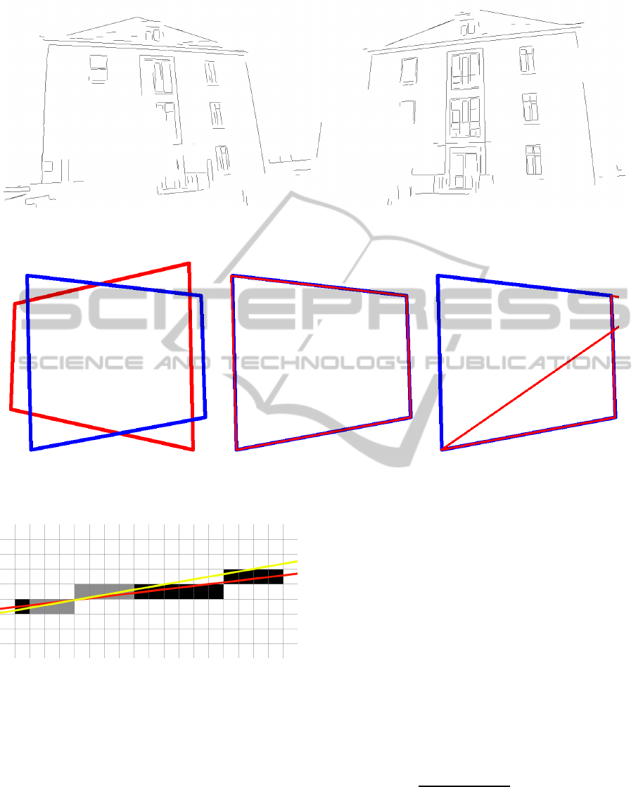
Figure 8: Two blueprints of the same building from slightly different views. The different occurrence of line segments is
obvious.
Figure 9: The left image shows two corresponding planes π and π
′
. The middle and the right image show the homography-
based transformation results with slightly wrong correspondence information. The point-based homography (middle) per-
forms still well while the line-based homography (right) fails.
Figure 10: A schematic representation of a line segment
(black) which is only covered partially by detected edge
points (gray). Obviously the underlying line for the black
line segment (red/dark) runs clearly different from the un-
derlying line of the gray line segment (yellow/bright).
5 THE PANNED ITERATION
LINE HOMOGRAPHY
ALGORITHM
We want to detect a facade F in both images I
1
, I
2
with
a homography. This can only work for plane facades.
We transform I
i
into two blueprints B
i
and apply the
following iteration algorithm lineHomography based
on panned line DLT.
We identify a blueprint B with its set of line seg-
ments. To a line segment s = p
1
p
2
with endpoints
p
1
, p
2
let l
s
= {(x, y) ∈ R
2
| xcosα + ysinα = d} be
the line through p
1
and p
2
in Hesse form. To any
line segment s we annotate its endpoints p
1
, p
2
and
the parameters α, d of l
s
. We thus can easily switch
from line segments to lines. We measure the distance
d(s
1
, s
2
) of two line segments by the distance of their
lines d(l
s
1
, l
s
2
) that is given as the differences of their
parameters α
i
and of d
i
. Since α and d have different
ranges we adapt these ranges, weight them equally
and scale the difference to [0, 1]. This is achieved
by d(s
1
, s
2
) =
|α
1
−α
2
|·f
r
+|d
1
−d
2
|
f
s
with a range factor
f
r
and a scale factor f
s
which depend on the image
size. Thus, even two disjoint line segments on dif-
ferent parts of the same line are in distance 0. d is a
metric on lines but not on line segments.
For a given homography H and threshold t we de-
note with C
H
the set of H-correspondences defined as
OnLine-basedHomographiesinUrbanEnvironments
365

C
H
:= {(s, s
′
) ∈ B
1
×B
2
|d(H(s), s
′
) < t}.
An H-correspondencesis thus a pair (s, s
′
) of line seg-
ments in B
1
and B
2
such that H maps s to a line seg-
ment close in distance to s
2
∈ B
2
.
5.1 Initial Line Segment
Correspondences
The first aim is to find an initial set C
init
of pairs of
line segment correspondences. This means to iden-
tify pairs of lines segments l
i
∈ B
1
and l
′
j
∈ B
2
which
describe the same line of the pictured object and lie
all on the same facade F in B
1
and B
2
. An auto-
matic detection of candidates of line on one facade is
in progress using of the known vanishing point but not
finished and implemented yet. Therefor, we manually
present C
init
. However, we also add some wrong cor-
respondences (l, l
′
) to C
init
where l and l
′
present dif-
ferent line segments in B
1
and B
2
on different facades
on different planes. Simply because no automated de-
tection of corresponding lines can avoid mistakes.
5.2 Panned DLT
We present the algorithm pannedDLT that will be
used frequently.
The input is a set C of 4 pairs of line segments
from B
1
×B
2
.
They posses 16 pairs of endpoints that are now
homogeneously panned. Homogeneously means that
the endpoints of the same line are panned in different
directions and that different line segments with a sim-
ilar direction are panned in the same way. This pan-
ning leads to 49 setsC
1
, ...,C
49
where eachC
i
consists
of supposed corresponding pairs of lines segments.
For any set C
′
of four corresponding pairs (s
1
, s
2
)
of line segments we regard the set
ˆ
C
′
of the four pairs
(l
s
1
, l
s
2
) of corresponding lines in their main form. We
now apply the line-based DLT to any set
ˆ
C
i
, 1 ≤ i ≤
49, where we use the parameters a, b, c for each line l
s
in
ˆ
C
i
. The resulting 49 homographies H
1
, ..., H
49
form
the output of pannedDLT with input C.
5.3 Line RANSAC
Hartley and Zisserman describe in chapter 4.8 of
(Hartley and Zisserman, 2004) the automatic compu-
tation of a (point-based) homography. An important
part of their proposed algorithm is the robust homog-
raphy estimation based on RANSAC which was pub-
lished by Fischler and Bolles in (Fischler and Bolles,
1981). We present here a RANSAC algorithm line-
RANSAC for lines based on panned DLT.
The input is a set C of n ≥ 4 pairs of corresponding
line segments in B
1
×B
2
.
Set j := 1,
repeat
create C
j
as a set of four randomly chosen pairs from
C,
compute 49 homographies H
j
1
, ..., H
j
49
from panned-
DLT with input C
′
j
,
compute the H
j
k
-correspondencesC
j
k
:= C
H
j
k
for 1 ≤
k ≤ 49,
j := j+ 1
until break (where break is a criterion as used usually
in RANSAC, depending on the average of the found
sizes of the sets C
j
k
).
Let j
0
be some index with
|C
j
0
| = max{|C
i
k
| | 1 ≤ i < j, 1 ≤k ≤ 49}.
RANSAC-step
Compute H by DLT with all correspondences in
ˆ
C
j
0
.
Obviously,C
j
k
consists of all inliers of the homog-
raphy H
j
k
. C
j
0
is a maximal set of found inliers in
the process. All its correspondences are now used to
compute a new homography H in the RANSAC-step.
5.4 RANSAC Line Homography
The input is C
init
as described in subsection 5.1.
Apply lineRANSAC with input C
init
to get the output
H and C.
C
new
:=
/
0,
repeat
C
new
:= C
new
∪C,
apply lineRANSAC with input C
new
to get the output
H and C
until a chosen number of iterations is reached or
C−(C∩C
new
) =
/
0.
The output of this ransacLineHomography algo-
rithm is the final homography H.
5.5 Line Homography
However, ransacLineHomography failes to give rea-
sonable homographies based on line correspon-
dences. It turns out that the RANSAC-step in 5.3 is
the reason: the DLT-algorithm with N > 4 line corre-
spondences is too unstable. We therefore have to drop
the RANSAC-step.
By lineHomography we denote the ransacLine-
Homography algorithm without the RANSAC-step in
5.3. The result of 5.3 is now the homography H
i
0
that gives reason to the maximal set C
i
0
of correspon-
dences.
VISAPP2013-InternationalConferenceonComputerVisionTheoryandApplications
366

5.6 Matching Decision
There are line segments in B
1
and in B
2
that we sup-
pose to lie on the same facade F presented as fa-
cade F
1
in B
1
and F
2
in B
2
. We choose an initial
defective set C
init
of pairs of corresponding line seg-
ments, apply lineHomography and result in a homog-
raphy H
final
. The correspondences which fit emi-
nently well to H
final
are used to hypothesize the lo-
cations of the main facades F(B
1
) and F(B
2
). This
is C
best
:= {(s, s
′
) ∈ B
1
×B
2
|d(H
final
(s), s
′
) < t
0
} for
a new threshold t
0
< t. C
1
best
consists of all line seg-
ments in B
1
that appear as a first coordinate in C
best
,
C
2
best
analogously are the line segments in B
2
appear-
ing in C
best
. CH
1
is the convex hull of C
1
best
and CH
2
that of C
2
best
. We map CH
2
by H
−1
final
in B
1
and set
CH
∩
1
:= CH
1
∩H
−1
final
(CH
2
). CH
∩
1
is used to process
the final evaluation.
Every line segment s of B
1
that lies inside CH
∩
1
is
projected to H
final
(s) in B
2
. We now compute a line
segment s
′
∈CH
∩
2
:= H(CH
1
) ∩CH
2
with a minimal
distance d(H
final
(s), s
′
). If this distance is below a
third threshold t
m
we regard s and s
′
a s a match. The
sum of all these distances per match is divided by the
number of all the matches to get the final error ε ∈
[0, 1].
If ε is smaller than a final fourth threshold t
f
:=
0.011 and a percentage ρ of at least 25% of all seg-
ments of B
1
within CH
∩
1
have found a match, F
1
and
F
2
are considered as a match of one and the same fa-
cade from different point of views. The two polygons
CH
∩
1
and CH
∩
2
form the assumptions of the facades
F(B
1
) and F(B
2
) in B
1
and B
2
.
6 EVALUATION
To evaluate our approach, we use 15 pairs of build-
ing images. Each pair shows among others the same
building facade from a different point of view. All the
images are recorded with the same SLR. By camera
calibration radial distortion is reduced in the images.
After applying the blueprint reconstruction algo-
rithm we posses a pair of blueprints B
1
and B
2
for
each image pair. In an evaluation set E
l
4
four cor-
rect line segment correspondences (s, s
′
) are anno-
tated to each pair of blueprints and furthermore, two
randomly generated incorrect line segment correspon-
dences. These six correspondences form the initial
correspondence set C
init
. In addition, we use a second
and third evaluation set E
l
6
and E
p
4
. In E
l
6
six correct
line segment correspondences and three incorrect line
segment correspondencesare used for each pair of im-
Table 1: The results of evaluation set E
l
4
with four correct
and two incorrect line segment correspondences. ε and ρ
are explained in chapter 5.6.
pair matched ε ρ match
lines
1 42 0.003681 35 1
2 17 0.006531 11 0
3 125 0.002412 34 1
4 50 0.001998 33 1
5 123 0.003005 27 1
6 100 0.002769 38 1
7 42 0.003102 45 1
8 19 0.002632 33 1
9 81 0.002694 35 1
10 61 0.004254 38 1
11 174 0.002942 37 1
12 87 0.003375 30 1
13 154 0.005112 41 1
14 25 0.006121 24 0
15 62 0.01051 59 1
mean 77 0.0041 35% 86.7%
ages. In E
p
4
only four correct point correspondences
are used.
As explained in 4.1 it is impossible in most in-
stances to find corresponding points in two blueprints.
Because of this the original image had to be used for
the annotation of the corresponding points in E
p
4
. It
should be noted that a creation of E
p
4
is much more
involved than of E
l
4
and E
l
6
.
We have run our algorithm lineHomography on
each C
init
of all the blueprint pairs of both evaluation
sets E
l
4
and E
l
6
and used the described matching deci-
sion. On E
p
4
the DLT has been run. In all three cases
the results are gained as described in chapter 5.6. Ta-
bles 1, 2 and 3 present the results.
The results for E
l
4
, E
l
6
, and E
p
4
are shown in table
1, 2, and 3, respectively. Because of the random steps
in our algorithm lineIteration the results per blueprint
pair of E
l
4
and E
l
6
vary in their quality and accuracy.
The evaluation runs presented in the tables are rep-
resentative but better and worse results are possible.
As all the image pairs contain in each case the same
building facade a 100% matching rate is desired.
E
p
4
produces the best results. As the DLT for
points is known to be stable and only correct corre-
spondences are used this is as expected and the results
may be considered as a standard. The desired match-
ing rate of 100% is reached, the absolute number of
matched line segments is the highest and ε is the low-
est.
Compared with these E
p
4
-results we consider the
results of E
l
4
and E
l
6
to be acceptable. The bad mean
ε of 0.0097 when using E
l
6
is caused only by one mis-
OnLine-basedHomographiesinUrbanEnvironments
367
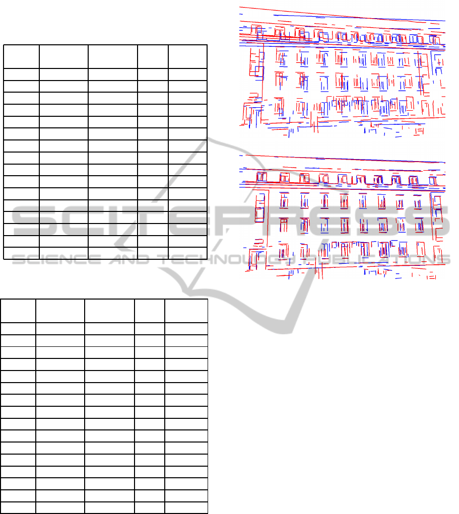
Table 2: The results of evaluation set E
l
6
with six correct
and three incorrect line segment correspondences. ε and ρ
are explained in chapter 5.6.
pair matched ε ρ match
lines
1 2 0.1018 12 0
2 69 0.003355 43 1
3 168 0.003023 40 1
4 44 0.001875 28 1
5 127 0.002635 28 1
6 95 0.00247 35 1
7 50 0.002869 48 1
8 34 0.002931 52 1
9 81 0.002098 35 1
10 62 0.003997 43 1
11 199 0.003061 45 1
12 67 0.004469 32 1
13 19 0.003671 19 0
14 101 0.002671 66 1
15 76 0.004361 46 1
mean 80 0.0097 38% 86.7%
Table 3: The results of evaluation set E
p
4
with four correct
point correspondences. ε and ρ are explained in chapter 5.6.
pair matched ε ρ match
lines
1 51 0.004077 38 1
2 61 0.004433 31 1
3 154 0.00282 35 1
4 51 0.002521 33 1
5 130 0.002739 27 1
6 97 0.002782 37 1
7 44 0.006547 49 1
8 34 0.003582 38 1
9 68 0.002414 30 1
10 68 0.003504 41 1
11 206 0.002802 40 1
12 111 0.003496 31 1
13 185 0.004673 48 1
14 85 0.003846 45 1
15 39 0.00458 60 1
mean 92 0.0037 39% 100.0%
match with a very high ε. E
l
6
has the same number of
mismatches, but both are only caused by few miss-
ing percentage points in ρ. However, the computation
time of E
l
4
and E
l
6
is much higher than of E
p
4
.
Figure 11 shows the two blueprints (upper image)
and the matched result (lower image) of image pair
no. 11 of E
l
4
. This is one example for the quality of
the results which lineIteration is able to produce.
Our blueprint approach provides a robust detec-
tion of line segments even in image regions with poor
Figure 11: Two different views of a building (upper image)
and the matching result (lower image) using line homogra-
phy with 4 correct and 2 incorrect line pairs initially.
textures. The results show that our approach states a
practical matching alternative in the absence of usable
or distinctive point features.
7 CONCLUSIONS
We have introduced a reconstruction of blueprints
from building images. We are quite content with this
algorithm and regard it as widely completed. The
blueprint forms a rather complex feature for image
analysis. We have used this feature for line-based
homographies that may be used for facade detection
e.g. The instability of line-based homographies is
well-known in the literature. Nevertheless, we suc-
ceed with our panned iterated algorithm in reasonable
results. These results are compareable with but not
as good as point-based results. On the other hand, it
seems to be easier to find initial line correspondences
with the help of blueprints than initial point corre-
spondences from the original image.
We still have to integrate a method for finding ini-
tial line segment correspondences automatically. Fur-
ther, we will include the Levenberg-Marquardt op-
timization algorithm as described in Appendix 6 in
(Hartley and Zisserman, 2004).
VISAPP2013-InternationalConferenceonComputerVisionTheoryandApplications
368

REFERENCES
Baltsavias, E. P. (2004). Object extraction and revision
by image analysis using existing geodata and knowl-
edge: current status and steps towards operational sys-
tems. ISPRS Journal of Photogrammetry and Remote
Sensing, 58(3-4):129 – 151. Integration of Geodata
and Imagery for Automated Refinement and Update
of Spatial Databases.
Bay, H., Ferrari, V., and Van Gool, L. (2005). Wide-baseline
stereo matching with line segments. In Proceedings
of the 2005 IEEE Computer Society Conference on
Computer Vision and Pattern Recognition (CVPR’05)
- Volume 1 - Volume 01, CVPR ’05, pages 329–336,
Washington, DC, USA. IEEE Computer Society.
Canny, J. (1986). A computational approach to edge de-
tection. IEEE Trans. Pattern Anal. Mach. Intell.,
8(6):679–698.
David, P. (2008). Detection of building facades in ur-
ban environments. In Rahman, Z.-u., Reichenbach,
S. E., and Neifeld, M. A., editors, Visual Information
Processing XVII, volume 6978 of Proceedings of the
SPIE, pages 69780P–69780P–11.
Dubrofsky, E. and Woodham, R. J. (2008). Combining line
and point correspondences for homography estima-
tion. In Proceedings of the 4th International Sympo-
sium on Advances in Visual Computing, Part II, ISVC
’08, pages 202–213, Berlin, Heidelberg. Springer-
Verlag.
Fischler, M. A. and Bolles, R. C. (1981). Random sample
consensus: a paradigm for model fitting with appli-
cations to image analysis and automated cartography.
Commun. ACM, 24(6):381–395.
Guerrero, J. and Sags, C. (2003). Robust line matching and
estimate of homographies simultaneously. In Perales,
F., Campilho, A., Blanca, N., and Sanfeliu, A., edi-
tors, Pattern Recognition and Image Analysis, volume
2652 of Lecture Notes in Computer Science, pages
297–307. Springer Berlin Heidelberg.
Hartley, R. I. and Zisserman, A. (2004). Multiple View Ge-
ometry in Computer Vision. Cambridge University
Press, ISBN: 0521540518, second edition.
Horowitz, S. L. and Pavlidis, T. (1976). Picture segmenta-
tion by a tree traversal algorithm. J. ACM, 23(2):368–
388.
Iqbal, Q. and Aggarwall, J. K. (1999). Applying perceptual
grouping to content-based image retrieval:building
images. In Computer Vision and Pattern Recogni-
tion, 1999. IEEE Computer Society Conference on.,
volume 1, Fort Collins, CO, USA.
Kumar, S. and Hebert, M. (2003). Man-made structure de-
tection in natural images using a causal multiscale ran-
dom field. In Computer Vision and Pattern Recogni-
tion, 2003. Proceedings. 2003 IEEE Computer Society
Conference on, volume 1, pages 119–126.
Leavers, V. F. and Boyce, J. F. (1987). The radon trans-
form and its application to shape parametrization in
machine vision. Image Vision Comput., 5(2):161–166.
L´opez-Nicol´as, G., Sag¨u´es, C., and Guerrero, J. J. (2005).
Automatic matching and motion estimation from two
views of a multiplane scene. In Proceedings of the
Second Iberian conference on Pattern Recognition
and Image Analysis - Volume Part I, IbPRIA’05, pages
69–76, Berlin, Heidelberg. Springer-Verlag.
Lowe, D. (2003). Distinctive image features from scale-
invariant keypoints. In International Journal of Com-
puter Vision, volume 20, pages 91–110.
M. Kuwahara, K. Hachimura, S. Eiho, and M. Kinoshita
(1976). Processing of ri-angiocardiographic images.
In Preston, K. and Onoe, M., editors, Digital Process-
ing of Biomedical Images, pages 187–202.
Mayer, H. (1999). Automatic object extraction from aerial
imagery–a survey focusing on buildings. Computer
Vision and Image Understanding, 74(2):138 – 149.
Priese, L. and Rehrmann, V. (1993). A fast hybrid color
segmentation method. In S.J. Pppl, H. Handels, edi-
tor, Proc. DAGM Symposium Mustererkennung, Infor-
matik Fachberichte, Springer Verlag, pages 297–304.
Priese, L., Schmitt, F., and Hering, N. (2009). Grouping
of semantically similar image positions. In Salberg,
A.-B., Hardeberg, J. Y., and Jenssen, R., editors, 16th
Scandinavian Conference, SCIA 2009, Oslo, Norway,
June 15-18, Proceedings, volume 5575, pages 726–
734.
Schmid, C. and Zisserman, A. (1997). Automatic line
matching across views. In Computer Vision and
Pattern Recognition, 1997. Proceedings., 1997 IEEE
Computer Society Conference on, pages 666 –671.
Schmitt, F. and Priese, L. (2009a). Intersection point topol-
ogy for vanishing point detection. In Accepted for
publication in: Discrete Geometry for Computer Im-
agery 2009, Montreal, Canada.
Schmitt, F. and Priese, L. (2009b). Sky detection in csc-
segmented color images. In Fourth International Con-
ference on Computer Vision Theory and Applications
(VISAPP) 2009, Lisboa, Portugal, volume 2, pages
101–106.
Zhang, W. and Koˇseck´a, J. (2007). Hierarchical building
recognition. Image Vision Comput., 25(5):704–716.
OnLine-basedHomographiesinUrbanEnvironments
369
