
A Predictive-Reactive Dynamic Scheduling under Projects’ Resource
Constraints for Construction Equipment
Mona Asudegi
and Ali Haghani
University of Maryland at College Park, College Park, U.S.A.
Keywords: Project Management, Dynamic Scheduling, Resource Constraints, Construction Equipment, Optimization.
Abstract: Major portion of projects’ cost is dedicated to construction equipment’s costs which signify the importance
of employing optimal equipment’s schedules in projects. In this paper the problem of construction
equipment scheduling for a company with several ongoing projects in different regions is studied. The goal
is scheduling heavy construction equipment and their assignments to jobs so that the total cost for the
company and disruptions in projects’ schedules is minimized while considering the priorities and critical
paths of the projects. A robust predictive-reactive integer model with a hybrid dynamic approach is
employed in modeling the problem. Case studies showed considerable savings in cost and minimizing
disruption in schedules in real time.
1 INTRODUCTION
Equipment scheduling problem is the problem of
allocating jobs to equipment over time. Since
availability of equipment and also jobs’ schedules
change during the projects, it is important to solve
the resource scheduling in projects dynamically.
Literature on dynamic equipment scheduling is very
sparse. Changes in resources or jobs could result in
dynamic characteristics of projects (Ouelhadj and
Petrovic, 2009).
A considerable number of studies have been
done on scheduling, but studies in construction
equipment scheduling are very rare (Słowiński and
Węglarz, 1989). In (Dodin and Elimam, 2008) a
static mixed integer model for scheduling equipment
based on tradeoffs among several costs is proposed;
however, a static model is not as efficient as
dynamic models in dynamic environment of
projects. Cost of ownership or renting construction
equipment such as cranes form main portion of
project costs. So implementing an optimal resource
management in construction industry is one of the
main ways in reducing costs. Moreover, Ernst et al.
(Ernst et al., 2004) highlights necessity of designing
mathematical models for each area of application
due to their unique characteristics. Here equipment
scheduling in the area of construction management
is studied.
2 PROBLEM STATEMENT AND
METHODOLOGY
2.1 Problem Statement and
Methodology
Large construction companies in the United States
and all over the world conduct several concurrent
projects at different sites in different locations, while
having a limited number of construction equipment
spread over the sites which are idle some of the time
during a project. Heavy construction machines are
highly costly and their ownership or rental cost
constitutes a significant portion of project cost.
Besides available owned equipment located in sites,
a company could use the option of renting similar
equipment from outside providers in different cities.
Schedule of the projects with the need of a specific
machine, and transportation network information is
assumed to be available in real time. The goal is to
solve the decision problem on using owned
equipment or rentals and to assign jobs to them in
order to maximize the benefit to the company. Some
assumptions are made through the study. Labours
are paid hourly and they do not cost when they are
idle. Rentals can be left at their job location after
finishing their task. Finally, rental and salvage price
during usage period is determined based on prices
on the start day of the task. The incorporated
notation is first shown below.
186
Asudegi M. and Haghani A..
A Predictive-Reactive Dynamic Scheduling under Projects’ Resource Constraints for Construction Equipment.
DOI: 10.5220/0004287003340337
In Proceedings of the 2nd International Conference on Operations Research and Enterprise Systems (ICORES-2013), pages 334-337
ISBN: 978-989-8565-40-2
Copyright
c
2013 SCITEPRESS (Science and Technology Publications, Lda.)

= Set of job site locations
, = Indices used for locations ,∈
= Set of works being done in site ∈
= Index used for works
= Index used for time (day)
= Beginning time of scheduling
1
= Latest time possible for starting work
= Earliest time possible for starting work
= Duration of work (in units of time)
= Travel time from location to location
= Transportation cost from location to
= Rental price from location for use in location
at time ($/day)
= Usage cost (depreciation cost) for an owned
equipment in location at time ($/day)
= Available owned equipment in at time
= Utility value of doing work at time ($)
Variables used in the model are as following.
1amachinefromlocationiassignedto
worknattimetinlocationj
0otherwise
1arentalmachinefromlocationi
assignedtoworknattimetinlocationj
0otherwise
Numberofavailablemachineswithnowork
assignedtoinlocationiattimet
The problem is modelled as a multi-objective model
incorporating several objectives as following.
i. Maximizing utility:
.
∈
∈
∈
(1)
ii. Minimizing transportation cost:
.
∈
∈∈
(2)
iii. Minimizing rental cost:
.
∈
∈∈
(3)
iv. Minimizing usage cost:
.
∈
∈∈
(4)
To combine all objectives, without loss of generality
it is assumed that they all have same weight and
importance for the company; however, knowing the
trade-offs between different objectives, the decision
maker can decide on the weight vector based on his
utility function by studying the Pareto set of
attributes (Bui and Alam, 2008). Following are the
constraints in the model.
∈
1;∀∈,∀∈
(5)
∈
∈
;∀∈,∀
(6)
∈
∈
∈
∈
;∀
∈,∀
(7)
0 ;∀∈,∀
(8)
,
;∀∈,∀∈,∀,∀∈
(9)
Constraints (5) enforce exactly one piece of
equipment being assigned to each job in the
acceptable time period. Constraints (6) assure not
sending more than available idle equipment from
each location to other locations. Constraints (7)
define the number of available idle equipment in
each location at each time period.
To define
, value of doing a job at time t, as
in (10), three factors are employed. First is cost and
penalty of conducting the work at any time other
than the planned schedule. This signifies the
difference between critical and non-critical jobs.
Second is the importance and priority of conducting
a job from the perspective of managers which can be
calculated using Analytic Hierarchy Process method
(Saaty, 1990). Third is the linkage between different
jobs due to the technical issues in a project.
0;
∑
∈
1
∗
∗
∑
∈
∗;
(10)
is set of all projects which project is one of
their predecessors.
is set of all projects which are
in need of the equipment at time t. 01 is the
project
’s importance index for the managers, and
is the budget assigned to project .
The predictive-reactive scheduling has two steps.
The model presented above generates a predictive
schedule employing available data in the first stage.
In the second stage, which can be repeated several
times, the original model is adjusted in order to
revise the schedule in response to real time events
and changes. In this stage notations are borrowed
from the first stage; however, the additional letter
“P” identifies updated information and the new set
of variables after rescheduling time (tp
0
in stage
APredictive-ReactiveDynamicSchedulingunderProjects'ResourceConstraintsforConstructionEquipment
187

two; e.g. TLP
n
is the updated latest starting time for
work n. The multi-objective function in the second
step contains additional elements as following.
i. Minimizing rental cancelation penalty:
.
0.3
∈|
|
,
∈
|∈
(11)
ii. Minimizing rental cancelation after equipment is
sent:
.
∈|
|,
∈
|∈
(12)
iii. Minimizing transportation cost due to job
cancelation:
.
∈
|,
∈
|∈
(13)
iv. Minimizing equipment schedules’ disruption due
to changes in schedules:
.
∈|
∈
|∈
(14)
Objective (11) minimizes 30% cancelation fee for
rentals scheduled for the next 48 hours in step one
which are cancelled in step two. Rental fee is
assumed not to be refundable after a shipment is
occurred in objective (12). Objective (14) minimizes
number of disruptions in the new schedule
comparing to step one’s schedule. Assigning
appropriate weights to different objectives and
summing them up, the problem would be a multi-
objective problem. An additional constraint (15), is
also added to the original constraints to assure no
equipment being assigned to the cancelled jobs.
∈
0;∀∈,∀
∈
|
0
(15)
Employing updated data into the new model a new
optimal schedule will be generated in stage two.
2.2 Numerical Analysis
The proposed dynamic model is applied on several
randomly generated examples with different
problem sizes; however, due to space limit, some of
the results are going to be discussed here. A set of
cases for a company with 25 site locations, 30 jobs,
and 100 day schedule is studied. Changes to the
projects are detected on day 40th including addition
of different number of new jobs. Projects’
information and resources data are exogenous and
generated randomly. Machine used in solving the
problem is a desktop computer with a 2.8 GHz CPU
and 1.99 GB of RAM. Xpress-IVE 7.0 is employed
as the optimization software.
Project’s cost for both dynamic and static models
for several randomly defined cases with different
number of additional jobs are compared in Figure 1.
In dynamic model, rescheduling is run when
changes are detected, while in static model
equipment are assigned to projects on a first come
first serve basis without considering optimal
reduction of cancelation penalties, unnecessary
transportation costs and delays in critical jobs. The
figure shows that applying rescheduling has reduced
costs in projects.
Figure 1: Effectiveness of rescheduling in reducing
projects' costs for several cases.
An interesting result from solving the model with
both binary variables and relaxed binary variables is
that although model’s coefficient matrix is not uni-
modular, both models give the same set of solutions
(Table 1). Interestingly enough, relaxing binary
variables which are the majority of the variables in
the problem does not improve the solution time
considerably. This might be due to dependency of
the node on which the algorithm is branching.
Another observation is that as the problem size
grows solution time increases significantly. Figure 2
illustrates sensitivity of solution time to time horizon
length in a case with 25 site locations and 5
additional jobs in the second stage. Results show, for
an average medium size problem, the dynamic
model can be solved in a reasonable amount of time
and is beneficiary to the economy of the project.
However, for a large size problem development of
an appropriate heuristic is inevitable.
ICORES2013-InternationalConferenceonOperationsResearchandEnterpriseSystems
188
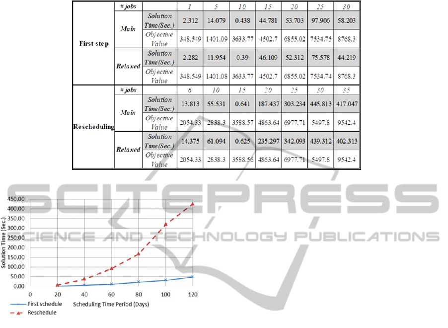
Table 1: Objective function and solution time for main and relaxed models.
Figure 2: Increase in solution time with the increase of
scheduling horizon, for 20 jobs in the first step.
3 CONCLUSIONS
In this study the problem of assigning and
scheduling construction equipment to jobs of several
projects over several sites of a construction company
considering the priorities and critical paths of the
projects is modelled as robust predictive-reactive
model. In the proposed dynamic model not only the
demands are satisfied and the cost is minimized, but
also interruptions in the project schedules due to
resource availabilities are minimized. The model is
capable of solving a moderate size problem in a
reasonable amount of time; however, dynamic
model makes it complex for large scale problems
and finding optimal solution would be challenging.
Designing an appropriate heuristic for large scale
problems and also considering stochastic nature of
projects is remained for future work.
ACKNOWLEDGEMENTS
Authors would like to thank FICO for kindly
providing the academic license of XPRESS-IVE 7.0
for this research.
REFERENCES
Bui, L. T. and Alam, S. (2008) 'An Introduction to Multi-
Objective Optimization', Multi-Objective Optimization
in Computational Intelligence: Theory and Practice,
1-19.
Dodin, B. and Elimam, A. A. (2008) 'Integration of
equipment planning and project scheduling', European
Journal of Operational Research, 184(3), 962-980.
Ernst, A. T., Jiang, H., Krishnamoorthy, M. and Sier, D.
(2004) 'Staff scheduling and rostering: A review of
applications, methods and models', European Journal
of Operational Research, 153(1), 3-27.
Ouelhadj, D. and Petrovic, S. (2009) 'A survey of dynamic
scheduling in manufacturing systems', Journal of
Scheduling, 12(4), 417-431.
Saaty, T. L. (1990) 'How to make a decision: the analytic
hierarchy process', European journal of operational
research, 48(1), 9-26.
Słowiński, R. and Węglarz, J. (1989) Advances in project
scheduling, Elsevier Science Ltd.
APredictive-ReactiveDynamicSchedulingunderProjects'ResourceConstraintsforConstructionEquipment
189
