
GPU Cost Estimation for Load Balancing in Parallel Ray Tracing
Biagio Cosenza
1
, Carsten Dachsbacher
2
and Ugo Erra
3
1
Universit¨at Innsbruck, Innsbruck, Austria
2
Karlsruhe Institute of Technology, Karlsruhe, Germany
3
Universit`a della Basilicata, Potenza, Italy
Keywords:
Ray Tracing, Image-based Techniques, Parallel Rendering, GPU.
Abstract:
Interactive ray tracing has seen enormous progress in recent years. However, advanced rendering techniques
requiring many million rays per second are still not feasible at interactive speed, and are only possible by means
of highly parallel ray tracing. When using compute clusters, good load balancing is crucial in order to fully
exploit the available computational power, and to not suffer from the overhead involved by synchronization
barriers. In this paper, we present a novel GPU method to compute a cost map: a per-pixel cost estimate of
the ray tracing rendering process. We show that the cost map is a powerful tool to improve load balancing in
parallel ray tracing, and it can be used for adaptive task partitioning and enhanced dynamic load balancing. Its
effectiveness has been proven in a parallel ray tracer implementation tailored for a cluster of workstations.
1 INTRODUCTION
Ray tracing algorithms (Glassner, 1989) model phys-
ical light transport by shooting rays into the scene
with the ultimate goal of producing photorealistic im-
ages. Considerable efforts have been made in order
to investigate new ways to reduce the high computa-
tional demands of ray tracing. Recent advances in ray
tracing include exploiting coherence between neigh-
boring pixels with packet traversal (Wald, 2004), ray
sorting (Garanzha and Loop, 2010), frustum traver-
sal (Reshetov et al., 2005), and fast updating of the
acceleration data structure for animated scenes (Zhou
et al., 2008; Cosenza, 2008). Thanks to recent im-
provements in both software and hardware, Whitted-
style ray tracing reaches interactive frame rates on
CPUs (Overbeck et al., 2008) and GPUs (Lauter-
bach et al., 2009). However, if we want to provide
more realism in the produced images, e.g. by com-
puting global illumination, we need to drastically in-
crease the number of secondary rays. Even though
several optimization strategies allow a certain amount
of interactivity, the use of complex rendering tech-
niques and shading algorithms, shadows, reflections
and other global illumination effects drastically in-
crease computation. The number of rays grows from
less than one million of typically coherent rays, up to
several millions (sometime even billions) of mostly
incoherent rays. In this context, distributing ray trac-
ing among several workers, i.e. multiple CPUs or
GPUs, is a viable solution to reach interactive frame
rates.
In this paper, we describe a GPU-based approach
for an efficient estimate of the per-pixel rendering
cost. The approach uses information available in the
G-Buffer generated by widely used deferred shading
techniques. By using the per-pixel rendering cost, we
are able to estimate the rendering time of any part of
the image generated by Whitted-style ray tracing or
path tracing.
A scenario where this approach would be use-
ful is a parallel ray tracing on clusters, where one
master node (equipped with a GPU) is responsible
for distributing tiles of an image (i.e. tasks) to sev-
eral worker nodes (equipped with multi-core CPUs or
GPUs) which perform ray tracing computation. In or-
der to have a good load balancing, the master node
tries to equally distribute tasks to each node minimiz-
ing the response time. Then, using our approach to
estimate the ray tracing cost of a tile of an image,
we can further improve task partitioning and dynamic
load balancing strategies.
We validate our idea by implementing a parallel
ray tracing system based on Whitted-style ray trac-
ing and path tracing that exploits the estimate of the
per-pixel rendering cost for balancing and distribut-
ing rendering tasks across workers in a network. We
perform the following steps to balance the rendering
139
Cosenza B., Dachsbacher C. and Erra U..
GPU Cost Estimation for Load Balancing in Parallel Ray Tracing.
DOI: 10.5220/0004283401390151
In Proceedings of the International Conference on Computer Graphics Theory and Applications and International Conference on Information
Visualization Theory and Applications (GRAPP-2013), pages 139-151
ISBN: 978-989-8565-46-4
Copyright
c
2013 SCITEPRESS (Science and Technology Publications, Lda.)
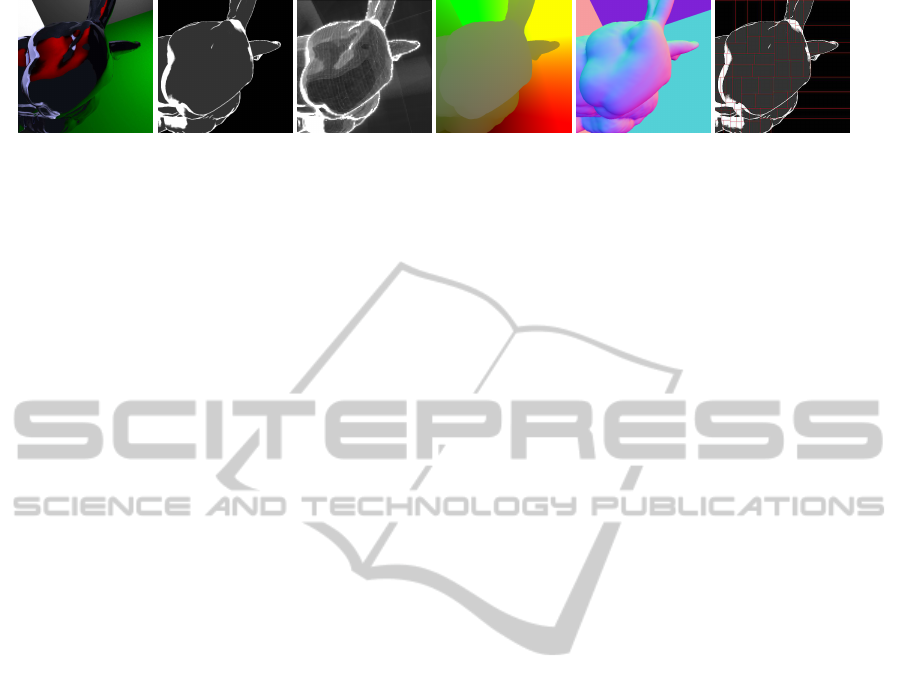
Figure 1: Left to right: the ray-traced image, the GPU-based estimation of the rendering cost, the actual packet-based render-
ing cost, position and normals in eye-space (used for the cost estimation), and using our method for an adaptive tiling of the
image for parallel rendering.
load:
1. Compute a per-pixel, image-based estimate of the
rendering cost, called cost map.
2. Use the cost map for subdivision and/or schedul-
ing in order to balance the load between workers.
3. A dynamic load balancing scheme improves bal-
ancing after the initial tiles assignment.
We show that the per-pixel cost estimate enables
good load balancing while maintaining a small num-
ber of tiles, thus allowing high rendering performance
even with slow networks.
2 PREVIOUS WORK
Ray tracing parallelization approaches can be clas-
sified into two main categories: image parallel de-
composition and scene geometry parallel decompo-
sition (SGPD), sometime referred as data paral-
lel (Chalmers and Reinhard, 2002). With image par-
allel methods, each worker is responsible for a region
of the image (e.g. a pixel or a tile), while the scene
data is usually (but not necessarily) replicated in the
memory of each node. On the contrary, in SGPD
methods, each worker is responsible for a part of the
scene, while rays propagate among the nodes. An im-
age parallel approach is typically the better solution
for scenes that can be stored in a single node as in our
case.
Early works in parallel ray tracing that reached in-
teractive performance used massively parallel shared
memory supercomputers (Muuss, 1995). Current
hardware trends in processor designs are turning to-
wards multi-core architectures and wide vector in-
structions. Manta (Bigler et al., 2006) is an inter-
active ray tracing system combining a high level of
parallelism with modern packet-based acceleration
structures. It uses a multi-threaded scalable paral-
lel pipeline in order to exploit parallelism on multi-
core processors. Similarly, (Georgiev and Slusallek,
2008) focuses on exploiting the massive parallelism
of multi-core hardware.
Ray Tracing on Distributed Memory Systems.
Developing interactive ray tracing for distributed
memory systems is an intricate process. Extend-
ing a renderer’s architecture to a cluster of work-
stations requires implementing several components,
such as a high-performance communication layer
and an efficient dynamic load balancer. Without
these techniques, the overhead of the communica-
tion causes poor scalability and performance penal-
ties. Commodity-based clusters offer a cost-effective
solution to speed up ray tracing, and many paral-
lel rendering frameworks as GigaWalk (Baxter et al.,
2002) or VR MantaJuggler (Odom et al., 2009) al-
ready support networked workstations.
Wald et al. (Wald et al., 2001) used coherent
ray tracing techniques in distributed memory archi-
tectures. Their system used a central server that takes
care of load balancing and stores the whole scene, but
they were able to render large and complex models at
interactiverates by using a two level BSP for per-node
caching of geometry. Later, several works improved
these techniques in order to render massivelycomplex
models (Wald et al., 2004; Dietrich et al., 2007). Dis-
tributed Shared Memory systems (DSM) offer a vir-
tual distributed memory address space in which each
node of a cluster has access to shared memory in ad-
dition to each node’s non-shared private memory. De-
Marle et al. (DeMarle et al., 2004), and more recently
Ize et al. (Ize et al., 2011), presented a state-of-the-art
read-only DSM ray tracer tailored for cluster hard-
ware. Our work is different in two aspects: We focus
on high-quality rendering using more involved algo-
rithms, such as path tracing, for scenes that can be
stored in a single node. Moreover our parallelization
approach is based on the message passing paradigm.
Budge et al. (Budge et al., 2009) introduced a sys-
tem that enables the rendering of globally illuminated
images of large, complex scenes by using a hybrid
CPU/GPU algorithm on a cluster. They developed an
efficient out-of-core data-management layer and cou-
pling this with an application layer containing a path
tracer.
Load Balancing. The major challenge of parallel
ray tracing on clusters is load balancing. In partic-
GRAPP2013-InternationalConferenceonComputerGraphicsTheoryandApplications
140

ular, if a rendering system is subject to a barrier syn-
chronization point (e.g., in synchronous rendering),
then the slowest task will determine the overallperfor-
mance. Achieving a good load balance is not trivial
and can be achieved using two main strategies: try-
ing to equally partition tasks, or using dynamic work
assignment.
Also choosing the number of tiles to subdivide the
image into (i.e. task granularity) is non-trivial. For
example, while a higher number of tiles facilitates
load balancing in a dynamic work assignment strat-
egy, it also results in a high number of communica-
tion, which is critical in networks with high latency.
Researchers have proposed many strategies for ad-
dressing load balancing in this context. Heirich and
Arvo (Heirich and Arvo, 1998) discussed the impor-
tance of dynamic load balancing for ray tracing in in-
teractive settings. Further related work examines the
importance of the subdivision granularity (Plachetka,
2002), and suggests adaptive subdivision to balance
the workload (Cosenza et al., 2008).
Although a demand driven centralized balancing
scheme achieves a well balanced workload, it in-
volves significant master-to-worker communication
which becomes a bottleneck when network transmis-
sion delay and the number of workers increase. A
decentralized load balancing scheme, such as work
stealing (Blumofe and Leiserson, 1999) or work re-
distribution, eliminates the communicationbottleneck
thus improving performance and scalability.
DeMarle et al. (DeMarle et al., 2003; DeMarle
et al., 2005) implemented a decentralized load bal-
ancing scheme based on work stealing. It is important
to notice that in their implementation, task migration
is done at the beginning of the next frame (frame-to-
frame steals), and the synchronization bottleneck at
the master node is hidden by an asynchronous task
assignment. Ize et al. (Ize et al., 2011) use a master
dynamic load balancer with a work queue comprised
of large tiles which are given to each node (the first
assignment is done statically and is always the same),
and each node has its own work queue where it dis-
tributes sub-tiles to each render thread.
More generally, the problem of load balancing is
very important for parallel rendering and visualiza-
tion and many solutions have been introduced, as for
instance using a kd-tree to divide the image into tiles
of equal cost (Moloney et al., 2007) or a cost esti-
mation based on the intersected primitives (Mueller,
1995).
Because of the higher load imbalance with more
involved rendering techniques (e.g. path tracing),
and because of the GPU availability on the master
node, we balance workload in a more effective way:
We implemented four different balancing strategies,
based on adaptive tiling, dynamic load balancing and
cost prediction, and we combine them with a multi-
threading parallelization based on tile buffering.
Rendering Cost Evaluation. Several factors affect
the rendering cost in ray tracing, such as scene size,
resolution, rendering technique, coherence between
rays, material properties, and the choice of the ac-
celeration data structure. In our context shading al-
gorithms affect the number of secondary rays traced
into the scene, and are the major cause load imbalance
among different pixels in the image (Figure 3).
Some techniques known in literature tackle the
problem of estimating the rendering cost. Gillibrand
et al. (Gillibrand et al., 2006) suggest that an approx-
imate render cost can be generated from a rasterized
scene preview. Profiling techniques are approaches
where the computation time of a small number of
samples (or pixels) is measured in order to have a
coarse approximation of the rendering cost.
While using a distributed memory architecture,
profiling is typically done on the master rather than
on the workers. If performed on the workers, sample
measures have to be sent back. Another issue is that
tracing few incoherent rays is slow. For these reasons,
we did not use profiling in our work. Beyond image-
space approaches, rendering cost estimation has been
explored even for SGPD (Reinhard et al., 1998).
An important remark is that our workload differs
from (Benthin et al., 2003) in two aspects: First, we
use Whitted ray tracing and path tracing instead of In-
stant Global Illumination; second, our test scene ex-
hibits high variance in shaders and geometry. Both
contribute to a high workload imbalance per pixel (as
shown by the real cost map in Figure 12), which is
challenging for system scalability. Our workload is
more similar to (Chalmers et al., 2006), where a paral-
lel selective renderer is used for physically-based ren-
dering.
3 THE COST MAP
In this section, we show how to obtain the cost
map, i.e. the image-based, per-pixel cost estimate
of the rendering process (see Figure 1 and Figure 2).
First, we define the problem statement and related ap-
proaches. Then, we introduce a GPU approach capa-
ble of quickly computing an approximate cost map,
and finally analyze the cost estimate error.
GPUCostEstimationforLoadBalancinginParallelRayTracing
141
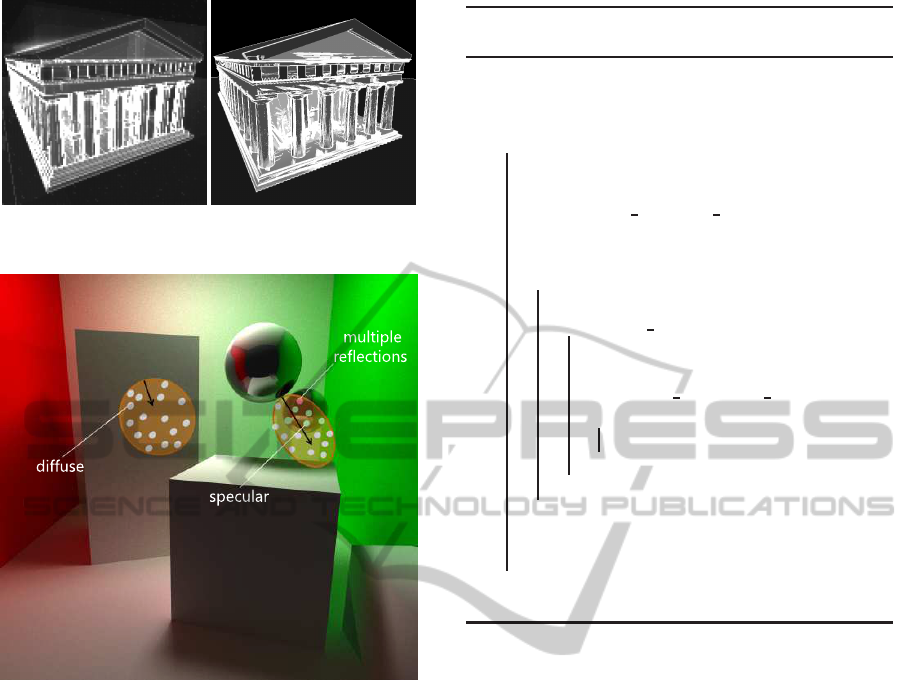
Figure 2: A comparison of the real cost (left) and our GPU-
based cost estimate (right).
Figure 3: Estimating the rendering cost: diffuse surfaces
typically have lower cost (in particular for Whitted-style
ray tracing), while specular surfaces generate more sec-
ondary rays thus causing higher rendering cost. Regions
where multiple reflections occur are typically more expen-
sive and can be found by a search in image-space. When us-
ing Monte Carlo-based techniques, the image-space search
can be adapted according to the specular coefficient of the
surface (see the sphere in the images).
3.1 The GPU-based Cost Map
To compute the cost map quickly on the GPU, we
make use of G-buffers known from deferred shad-
ing (Hargreaves, 2004) and image-space sampling.
The underlying idea is that it is often possible to de-
tect potentially expensive areas, e.g. with multiple in-
terreflections by solely performing a search for such
geometric configuration using image-space informa-
tion.
Algorithm 1 describes our image-based technique,
assuming that the properties of each pixel belonging
to a visible surface are available.
Algorithm 1: Approximated cost map computation
algorithm. Code for pixel P
i
.
1 // All the data of the hit surface on the pixel P
i
are available
2 cost
i
← basic material cost of the hit surface ;
3 if P
i
is reflective then
4 // Determinate the sampling pattern S, at
the point P
i
, toward the reflection vector R
5 S = compute sampling pattern(P
i
,R) ;
6 // For each samples, calculate cost
contribute
7 for each sample S
j
in S do
8 sample
j
← 0 ;
9 if visibility check(S
j
,P
i
) then
10 increase sample
j
;
11 if
secondary reflection check(S
j
,P
i
)
then
12 increase sample
j
;
13 end
14 end
15 end
16 // Samples gathering
17 cost
i
= cost
i
+ gather(S) ;
18 end
19 return cost
i
We assign a certain basic cost to each pixel P
i
de-
pending on its material, e.g. the cost for evaluating
the BRDF model. Next, if the surface is reflective,
we perform an image space search in order to de-
tect potentially expensive areas, e.g. where multiple
interreflections are likely. To this end, we create a
set of samples which are used to obtain the informa-
tion about the surfaces from the G-buffer. We use an
initially uniformly distributed set of sampling points
which is transformed before sampling (line 5). This
transformation is computed according to the reflec-
tion properties of the surfaces (mainly glossiness), the
rendering technique (Whitted-style raytracing, path
tracing etc.) and oriented along the reflection vector
R projected into image space.
Intuitively, the pattern is scaled to become more
narrow for surfaces with higher specularity, and posi-
tioned at the surface point P
i
in question and oriented
along the projection of its reflection vector (Figure 3).
For every sample S
j
, we retrieve its surface loca-
tion and orientation from the G-Buffer. Next, we per-
form a test to detect the sample cost: We test if P
i
and
S
j
are mutually front-facing (line 9). Later, a test de-
tects if the sampled surface is reflective (line 11). If
the surface at S
j
is reflective, and the lobe of specular
reflection of S
j
points towards P
i
then we detected a
region with a potentially high number of interreflec-
GRAPP2013-InternationalConferenceonComputerGraphicsTheoryandApplications
142

tions, and further increase the cost estimate. After the
sampling phase, we gather the contributions from all
samples.
Sampling Pattern. The sampling pattern evaluated
by compute
s
ampling
p
attern(P
i
,R) (see Figure 4) is
randomly generated (a) and scaled (b) according to
the surface properties. Essentially, the pattern is trans-
lated (c) and rotated (d) to align with the reflection
vector R. Step (b) depends on the material as well as
the rendering technique. In particular, we distinguish
a wider sampling pattern for Lambertian and glossy
surfaces for path tracing, but the pattern collapses to
a line for Whitted-style ray tracing and for path trac-
ing using a perfect mirror material. The sampling for
the cost map computation is performed only once per
pixel, not recursively.
Sample Gathering. Once sampling has been per-
formed, we gather the contributions from all sam-
ples. This step is somewhat correlated to the ren-
dering technique. In particular, the final cost may be
computed in two ways: by summing up the sample
contributions, or by taking their maximum. The first
approach is used in path tracing, where we suppose
that secondary rays spread along a wide area. In the
contrary, when using Whitted ray tracing, all samples
belong to one secondary ray and we conservatively
estimate the cost by taking the maximum.
Edge Detection. Real-time ray tracers use bundles
of coherent rays, called ray-packets, to achieve real-
time performance on CPUs (Wald, 2004; Overbeck
et al., 2008). Whenever packet-based ray tracing is
used, packet splitting raises the cost because of the
loss of coherence between rays. This occurs at depth
discontinuities that we detect by using a simple edge-
detection filter on the G-Buffer. By further increasing
the cost estimate at edges, we account for the impact
of packet splitting. We experienced that this extra cost
is significant only with Whitted ray tracing.
Implementation Details. The algorithm has been im-
plemented in a two pass shader. In the first pass, we
render the scene to a G-Buffer using multiple render
targets to store data. For every pixel, we store the
position, the normal, and a value indicating if the sur-
face is reflective, for the first visible surface seen from
the camera (Figure 3). We also store three additional
values: The basic shader cost, the specular coefficient
and the Phong exponent. In the second pass, we gen-
erate the cost map using the image-space information
stored in the G-Buffer. The basic value has been used
in several points of the algorithm (i.e. lines 2 and 10).
The other values both are required in the sampling
phase (line 5 and Figure 4). Details about rendering
parameters are shown in Table 1. The memory re-
quired by the algorithm amounts to three screen-sized
textures used by the G-Buffer (in our implementation,
three 512
2
floating-pointRGBA textures, i.e. 12 MB).
The cost map generation is fast: Whereas both
CPU and GPU computation take less than 1 ms, the
most expensive task is the data transfer between GPU
and CPU (5-6 ms). However, this time is spent by
the master node in barrier, i.e. when preparing the
cost map before distributing the work load. For that
reason, this time is further hidden using an pipelined
prediction optimization (details in Section 5).
3.2 Cost Estimation Error Analysis
The resulting cost map is obviously approximate. We
analyzed the error in order to understand where and
why the estimate is accurate and where not. Because
of the use of ray-packets, our analysis is performed
at packet-level instead of pixel-level. First, we mea-
sure the difference between the approximate cost and
the real cost (packet-based error) for each ray-packet.
Second, we analyze difference maps of real and ap-
proximate cost to be thoroughly aware about where
the estimate is less accurate. In the subsequent sec-
tions, we analyze the performance of a parallel ray
tracing system, evaluating how much the cost map en-
ables better task distribution to several worker nodes
by using two balancing techniques.
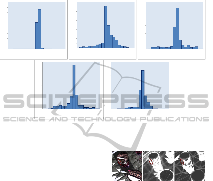
Five test scenes (Figure 5) have been used to eval-
uate the estimate of the cost map. In Figure 6, we
show the error distribution of the (packet-based) dif-
ference between the real computing time and the es-
timated one. The analysis shows that the estimate is
quite accurate, and errors usually lead to an under-
estimation, caused by the off-screen geometry prob-
lem. Because our strategy works on a rasterized scene
preview, our algorithm only works on visible geome-
try. Nevertheless, reflected rays may fall in geometry
not present in the frame buffer. When this happens,
the algorithm is not able to detect a reflected surface
and the resulting calculated cost is under-estimated in
respect to the real one (Figure 7).
For instance, in the case of the Cornell box scene,
the cost estimation is quite accurate: the 86% of
the predictions fall in the first approximation interval
(+/ − 5% of the real packet time). Note that the 87%
of the predictions are under-estimated (error ≥ 0). In
the contrary, the Ekklesiasterion scene is less accu-
rate: only the 57% have a good approximation. Here,
84% of the predictions are under-estimated. Figure 12
shows real cost and GPU-calculated cost maps, and
the difference between real and approximate cost.
Note that we can reduce the off-screen problem by
GPUCostEstimationforLoadBalancinginParallelRayTracing
143
R
(a) (b) (c) (d)
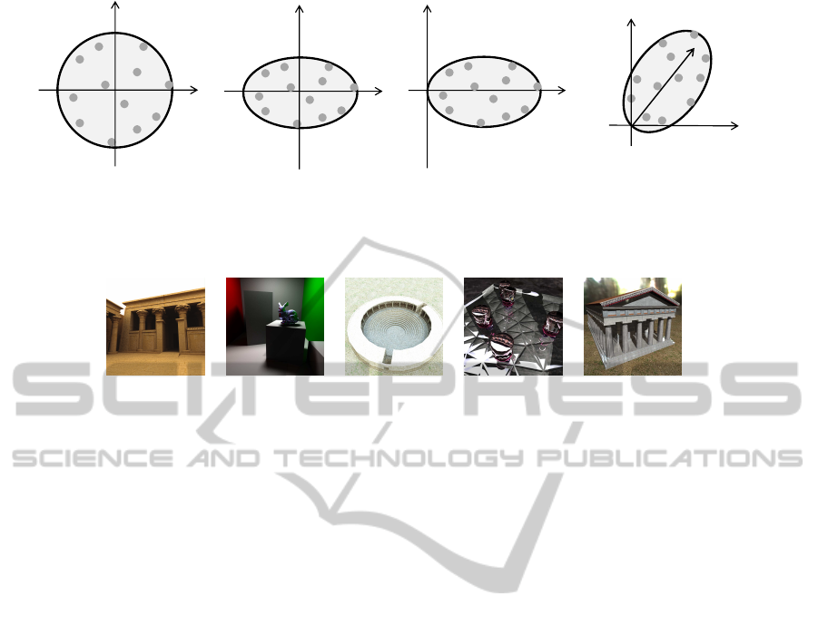
Figure 4: Sampling pattern. The sampling patterns used in the cost map generation algorithm. At first, an uniformly distributed
set of points is generated (a). According to the shading properties, the pattern is scaled (b) and translated to the origin (c). In
the last step, it is transformed according to the projection of the reflection vector in the image plane(d).
Kalabsha Temple Cornell box Ekklesiasterion Toasters Paestum Temple
Figure 5: Our test scenes. Rendering parameters are shown in Table 1.
computing the cost map for an extended image plane
to capture surfaces outside the current view. The use
of the A-buffer would further guarantee that the whole
geometry is available on the render buffer (Carpen-
ter, 1984), and it requires only a fixed amount of
GPU memory that increases linearly with image space
size (Yang et al., 2010). One limitation of our imple-
mentation is that the scene should fit into the GPU
memory. However, because we use the GPU only for
the cost map computation (i.e. does not affect the
final rendering), one could easily use low-resolution
meshes or level-of-detail approaches for the GPU cost
map estimation, which might then be slightly less ac-
curate.
4 LOAD BALANCING
In this section, we describe how we use the cost map
for two different load balancing strategies. In order
to exploit the cost map, we use a Summed Area Ta-
ble (Crow, 1984) created on the GPU. Summed Area
Tables (SATs) allow us to compute the sum of values
in a rectangular region of an image in constant time.
A SAT of the cost map allows us to directly compute
the cost estimate for an image tile. Given a cost map
of dimension n × n (where n is the number of pixel
per dimension), we can compute a SAT directly on
the GPU in O(logn) time (Hensley et al., 2005).
SAT Sorting. An immediate use of the SAT is to
compute the cost of a tile after subdividing the image
in equally sized tiles. Next, we can sort the tiles for
decreasing cost, assuring that computationally more
expensive tiles are scheduled before cheaper ones.
The reason for this approach is that dynamic load bal-
ancing typically works better if nodes work on more
expensive tasks at first, and task transfers or steals
are performed for smaller tasks afterward (e.g. chunk
scheduling (Grama et al., 2003)).
SAT Adaptive Tiling. We can alternatively use the
SAT to determine an adaptive subdivision of the im-
age space into tiles of roughly equal cost. Our adap-
tive subdivision algorithm can be seen as a weighted
kd-tree split using the SAT to locate the optimal splits.
In our implementation we use two temporary de-
ques (double-ended queues), P and Q, and the cost
map C and the number of iterations l as input. During
subdivision, we use Q to store the current tiles to be
split, and P to store the tiles that have already been
split. The resulting subdivision of our algorithm is
well balanced and all tiles exhibit almost equal cost
(see Algorithm 2).
5 PARALLEL RAY TRACING
In this section, we briefly discuss the main challenges
of our parallel ray tracing system: the tile-to-packet
mapping, the dynamic load balancing, and further op-
timizations. In order to validate the use of the cost
map, we implemented Whitted-style ray tracing and
path tracing.
Our implementation of the work assignment,
scheduling, and dynamic load balancing is decoupled
from the ray tracing implementation that runs on the
GRAPP2013-InternationalConferenceonComputerGraphicsTheoryandApplications
144
0K
20K
40K
60K
80K
100K
120K
140K
160K
180K
-50
-45
-40
-35
-30
-25
-20
-15
-10
-5
0
5
10
15
20
25
30
35
40
45
50
Cornell box
0K
10K
20K
30K
40K
50K
60K
70K
80K
90K
100K
-100
-90
-80
-70
-60
-50
-40
-30
-20
-10
0
10
20
30
40
50
60
70
80
90
100
Ekklesiasterion
0K
20K
40K
60K
80K
100K
120K
-20
-18
-16
-14
-12
-10
-8
-6
-4
-2
0
2
4
6
8
10
12
14
16
18
20
Toasters
0K
20K
40K
60K
80K
100K
120K
-20
-18
-16
-14
-12
-10
-8
-6
-4
-2
0
2
4
6
8
10
12
14
16
18
20
Paestum Temple
0K
20K
40K
60K
80K
100K
120K
140K
-50
-45
-40
-35
-30
-25
-20
-15
-10
-5
0
5
10
15
20
25
30
35
40
45
50
Kalabsha Temple
Figure 6: Error distribution of the estimation. Each packet-based rendering time is subtract from the cost map estimate, for
the same corresponding packet of pixels. The x-axis shows the difference in error intervals, from negative values (left, over-
estimation) to positive ones (right, under-estimation). The y-axis plots error occurrences for each error interval. Tests have
been performed on one Intel Pentium IV CPU 3.40GHz with 2048KB cache size, averaged for a walk through of few frames
in the scene.
individual worker. We base our ray tracing imple-
mentation on Manta (Bigler et al., 2006), which we
extended with new image traversal algorithms, load
balancers, shaders, and by adding new components.
In particular, our parallel code is hidden behind the
traversal logic, with a master-side and a worker-side
component. The first is responsible for the prediction
and assignment, and implements a GPU-based ren-
dering system with programmable shaders. The latter
hides the CPU-based ray tracing system and the dy-
namic distributed load balancer. A material table is in
charge of linking the ray tracer shading information
with the GPU-cost map generation. As we use static
scenes, we employ precomputed kd-trees built with a
SAH metric as acceleration data structure.
Tile-to-Packet Mapping. As we discussed before,
we use a ray tracer which bundles coherent rays to-
gether to ray-packets. The packeting size is usually
set to a value that enables exploit SIMD units and op-
timize data locality. Recent approaches encourage the
usage of large ray packets for Whitted-style ray trac-
ing (Overbeck et al., 2008).
The use of two different levels of parallelism, one
being the packets of the ray tracer, and one being the
splitting of the image into tiles, raises the problem of
how to map a tile to packets. The optimal packet size
Figure 7: Off-screen geometry problem. The image indi-
cates an area where secondary rays fall outside geometry in
the rendering buffer (a), hence raising the cost of these pix-
els (b). Our GPU technique under-estimates the cost of this
area (c).
mainly depends on the scene, the acceleration data
structure, and the hardware architecture. Similarly,
a parallel distributed memory system has an optimal
task (i.e. tile) size that depends on the ratio of compu-
tation to the amount of communication, being critical
in systems like a cluster of workstations. Fixing the
same task size for both with an one-to-one approach
does not reach optimal performance of the whole sys-
tem. A one-to-one approach also complicates, and
limits, the exploitation of the cost map for adaptive
subdivision. Our system uses a one-to-manyapproach
instead: each tile is subdivided into packets of fixed
optimal size, e.g. each tile is subdivided in packets of
8×8 rays per packet. Ize et al. (Ize et al., 2011) used
a similar two-level load balancer in their DSM-based
GPUCostEstimationforLoadBalancinginParallelRayTracing
145
implementation, but in our work, the first level load
balancer is based on work stealing (i.e. distributed
load balancing).
Algorithm 2: The SAT-tiling algorithm. Starting
with a single tile covering the entire image (i.e. of the
same size as the cost map), each iteration chooses a
split-axis and subdivides the tile two tiles T
1
and T
2
,
with approximately the same cost. The running time
is O(n
2
), where n is the number of pixel per dimen-
sion.
1 // Set the first split axis (0=x-axis, 1=y-axis)
2 Axis ← 0 ;
3 // Create and enqueue the initial tile (covering
the entire image) to P
4 Enqueue(P, CreateTile()) ;
5 // Loop l times to obtain 2
l
tiles
6 for i ← 0 to l do
7 // Q contains all tiles to be split
8 Q ← P ;
9 // P stores the newly split tiles
10 P ←
/
0 ;
11 while Q 6=
/
0 do
12 // Remove a tile T from the queue
13 T ← Dequeue(Q) if axis = 0 then
14 (T
1
,T
2
) ← SplitX(T) ;
15 else
16 (T
1
,T
2
) ← SplitY(T) ;
17 end
18 // Enqueue two tiles T
1
and T
2
and
select the next split axis
19 Enqueue(P, T
1
) ;
20 Enqueue(P, T
2
) ;
21 Axis ← 1 - Axis ;
22 end
23 end
Work Stealing. Our parallel system performs in-
frame steals to improve the load balancing computed
from the cost estimation. Note that a perfect cost
map would make work stealing superfluous; how-
ever, this cannot be expected from an image-space
estimation. Our work stealing implementation fol-
lows the scheme suggested in (Blumofe and Leiser-
son, 1999) where each worker has a queue
1
: each
worker first processes his own tasks starting from the
top of his queue. When the queue is empty, work-
ers start stealing tasks from another randomly chosen
worker (Figure 8). Although dynamic load balancing
1
We adopt the terminology of (Blumofe and Leiserson,
1999) using the word queue. However, as our work steal-
ing algorithm performs operations in both the top and the
bottom of the queue, the correct term would be deque.
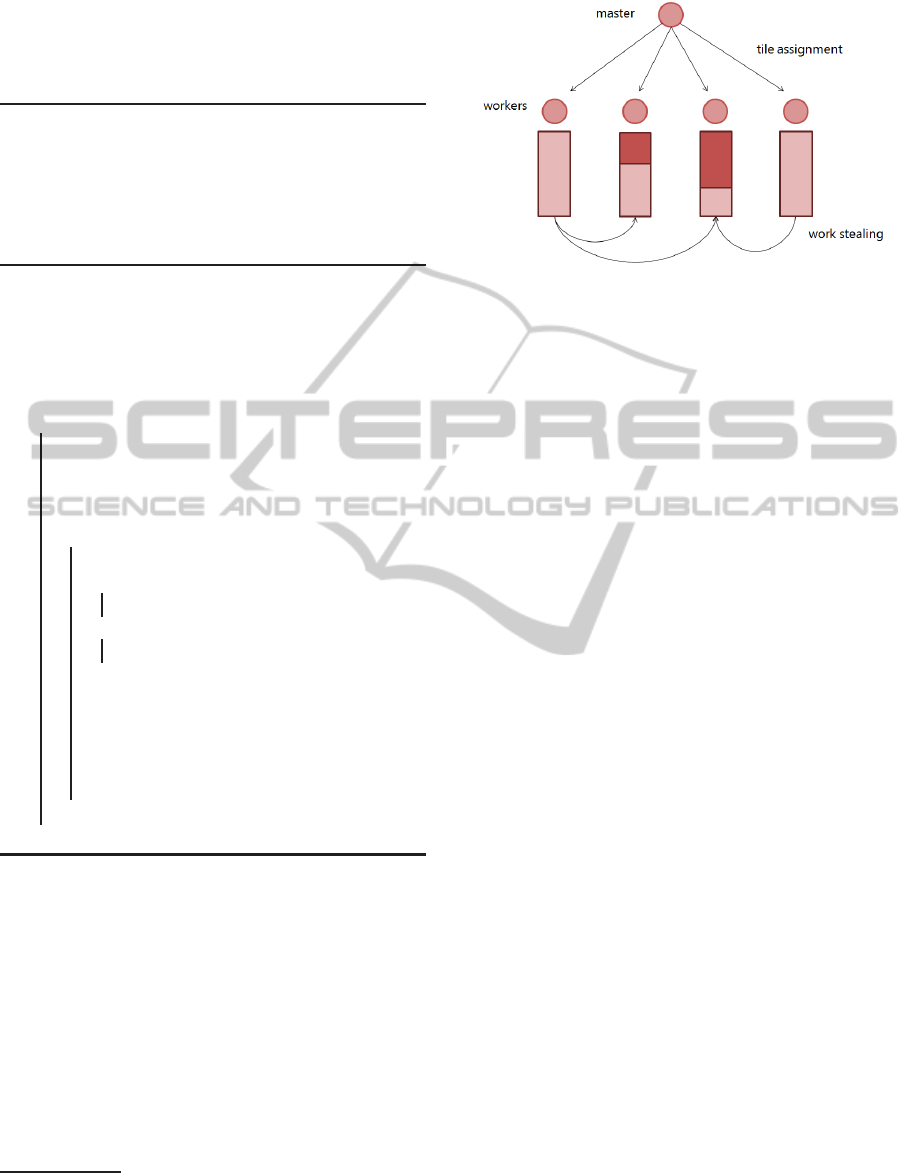
Figure 8: A master node is responsible for the first task
assignment. Using work stealing idle workers search among
the other workers in order to find unprocessed tiles.
is distributed, first task assignment is centralized. All
tiles are assigned at the beginning of the frame by the
master node, using prefetching to hide latency (i.e. by
assigning all the tiles at once, without any on demand
request from the workers) and assuring fairness (i.e.
preventingstarvation of MPI processes). Then the dy-
namic distributed load balancing algorithm takes care
of an initially unbalanced work distribution. Further
optimizations in the work stealing protocol can save
communication when, for instance, two nodes send
crossed steal requests (i.e. avoiding to send two neg-
ative ack messages). An important aspect when im-
plementing in-frame steals is to take care of the frame
synchronization barrier. A node entering into stealing
mode performs steal requests until a new frame starts.
The new frame message, however, is sent by the mas-
ter node without a guarantee for order-preserving and
delivery, i.e. it may happen that a node at frame f + 1
receives an old steal request sent by a node at the
frame f. We solve this problem by adding the frame
number to the steal request and steal ack messages.
Further Optimizations. On each node, the ray trac-
ing itself can also be parallelized via multiple threads
and ray packets, e.g. if multi-core CPUs and SIMD
instruction sets are available. On top of Manta, our
distributed parallel architecture introduces the queue
of tiles as an additional element to support work steal-
ing. Moreover, a tile buffer has been introduced to
efficiently support multi-threading. Figure 9 shows
how the tile buffer is integrated with the work steal-
ing queue.
We utilize MPI as a means to exchange data be-
tween nodes. Our system hides latency by implement-
ing task prefetching and using asynchronous data
transfer where possible. At the beginning of each
frame, the camera position and a list of prefetched
tiles is sent to each worker.
The overhead introduced for generating the cost
map, the SAT and to compute the tiling causes a
GRAPP2013-InternationalConferenceonComputerGraphicsTheoryandApplications
146
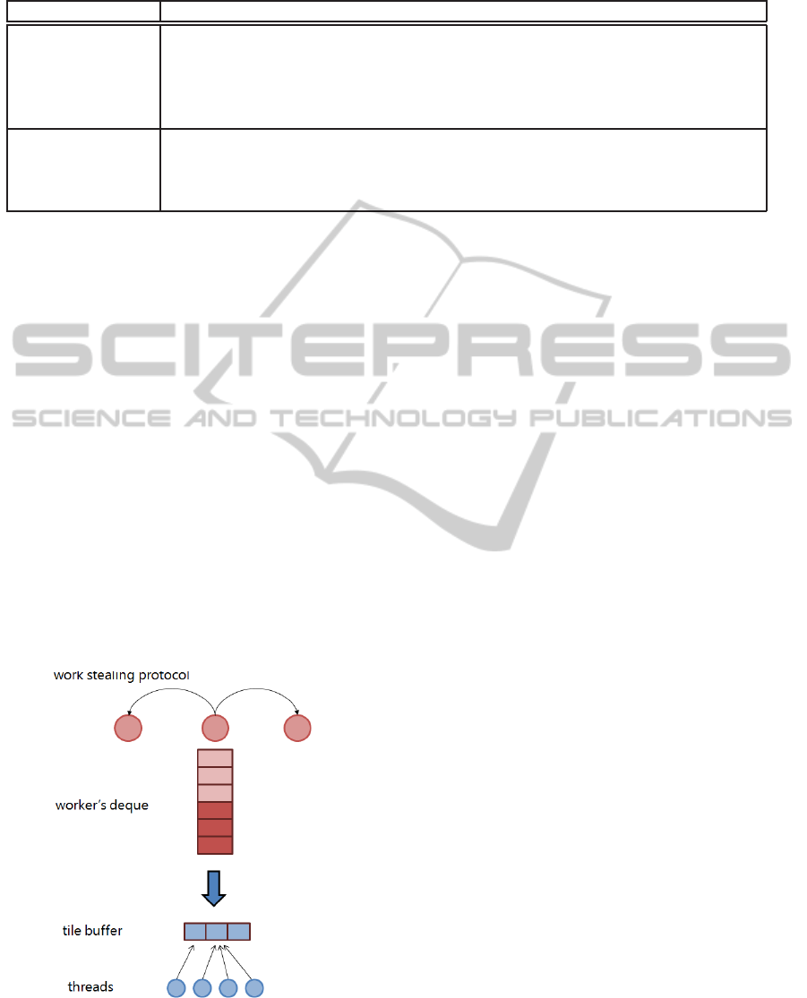
Table 1: Summary of the parameters used for rendering and cost map computation. The packet size is the optimal value for
each test scene.
Scene Kalabsha temple Cornell box Ekklesiasterion Toasters Paestum temple
# triangles 4529462 69495 3346 11141 13556
Rendering tech. path tracing path tracing path tracing whitted whitted
Rays/pixel 128 jitter 128 jitter 32 jitter 8 jitter 1
Packet size 8 8 16 16 32
Primary rays 134.2M 134.2M 33.6M 8.4M 1.0M
Sampling pattern wide pattern wide pattern wide pattern collapsed collapsed
to a line to a line
Edge detection no no no yes yes
Samples gathering sum sum sum max max
longer barrier. We hide this overhead by means of a
pipelined prediction: after the task assignment for the
frame f, when all workers are busy, the master node
starts computing the prediction for the frame f + 1.
The overall architecture is still synchronous, whereas
just the prediction phase is computed asynchronously.
6 RESULTS
We ran several benchmarks on a test platform consist-
ing of a cluster of workstations equipped with Intel
six-core Xeon X5650 CPUs running at 2.7 GHz and
24 GB DDR3 ECC RAM. Nodes are interconnected
with an Infiniband network. The master and visu-
alization node is equipped with an NVidia GeForce
GTX 570. The cost map computation has been imple-
mented using OpenGL and GLSL. Running the mas-
ter and the worker node on a single host may reduce
Figure 9: Multi-threading with tile buffering. A small num-
ber of tiles moves from the queue to the buffer. This al-
lows separating the work stealing algorithm, working on the
queue, from the multi-threading parallelization, working on
the tile buffer.
performance. For this reason, we used a specific vi-
sualization host as the master node.
Test scenes. All images have been rendered at a reso-
lution of 1024×1024pixels, with 128 tiles and a max-
imum recursion depth of 4, resulting in highly vary-
ing rendering cost in regions with interreflections.
Pipelined prediction has been enabled in all tests. In
order to study the impact of our techniques, we used
five different test scenes (Figure 5), having different
rendering parameters, rendering techniques and over-
all workload: The first three scenes use path tracing
and thus are computationally more expensive. The
first is the Kalabsha temple. For each pixel, we apply
a jitter pattern of 128 rays/pixel, shooting 134.2 mil-
lion of primary rays. We used the same parameters
for the second scene, a Cornell box with a reflective
Bunny and an area light. The Ekklesiasterion scene
contains an ancient Greek building. For this scene,
we used 32 rays/pixel. The other two test scenes
were rendered using Whitted ray tracing with respec-
tively 8 and 1 rays/pixel. The Toaster and Poseidonia-
Paestum temple both present a large number of re-
flective surfaces. Table 1 shows ray-packet size, the
number of primary rays, and the rendering parame-
ters used for each test scene. We performed scalabil-
ity tests by using up to 16 workers; each worker uses
6 threads.
For each test scene, we show results using 4 dif-
ferent balancing approaches: A simple unbalanced
approach without dynamic load balancing and using
equally sized tiles (Regular without WS); a regular ap-
proach using work stealing for load balancing (Regu-
lar); an adaptive approach using the SAT of the cost
map and work stealing (SAT Adaptive); a sorting-
based approach using SAT and work stealing. For all
approaches, there is an initial tiles assignment phase
where each node gets a set of tiles that are close in im-
age space. Table 2 shows performance for 16 workers
and shows the parallel speedup and efficiency.
An analysis of the number of steal transfers is
shown for all the test scenes in Figure 10. This analy-
GPUCostEstimationforLoadBalancinginParallelRayTracing
147
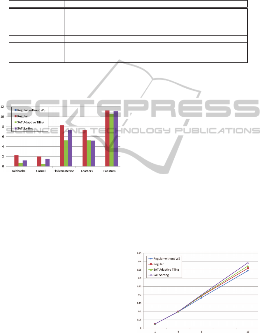
Table 2: Performance comparison for our five test scenes; timings are given in seconds per frame. We report speedup and also
efficiency which describes the fraction of the time that is being used by the processors. Tests have been performed with 16
workers and multi-threading.(*) Speedup and efficiency is shown for Regular without WS and SAT Sorting approach.
Scene Kalabsha temple Cornell box Ekklesiasterion Toasters Paestum temple
Regular without WS 5.285 2.901 0.765 0.067 0.0126
Regular 4.862 2.783 0.750 0.066 0.0112
SAT Adaptive Tiling 4.889 2.680 0.745 0.064 0.0108
SAT Sorting 4.542 2.548 0.638 0.059 0.0102
1 worker 70.639 40.005 9.391 0.932 0.154
Speedup* 13.4 - 15.6× 13.8 - 15.7× 12.3 - 14.7× 13.9 - 15.8× 12.2 - 15.1×
Efficiency* 83 - 97% 86 - 98% 76 - 91% 86 - 98% 76 - 94%
+16% +13% +19% +13% +23%
sis is helpful to understand how different tiling algo-
rithms work and, once an initial tile set is assigned,
how balancing algorithms integrate with work steal-
ing algorithms.
Figure 10: Steal transfers. The graph shows the average
number of steal transfers performed during our test, using 4
workers. Note that a node may steal even more than one tile
per frame. Note, the regular approach does not use work
stealing.
7 DISCUSSION
Our analysis of the results focuses on the effectiveness
of the load balancing techniques utilized (SAT Adap-
tive Tiling and SAT Sorting), their correlation with
the approximation of the cost map, and scalability.
SAT Adaptive Tiling. Our results show that the
Adaptive Tiling is similar in performance to the Regu-
lar approach. However, it never outperforms the SAT
Sorting approach. The steal transfers analysis (Fig-
ure 10) reveals additional information. An important
issue is that the number of steal transfers of adaptive
tiling is often the lowest. This means that (1) the ini-
tial tile assignment provided by the adaptive tiling is
more balanced than the regular one; (2) work steal-
ing does not work well with such kind of (almost bal-
anced) workload. In fact dynamic load balancing, in
our case the work stealing strategy, rivals adaptive
tiling since both try to balance the workload: a fine
grained balancing with dynamic techniques requires
more expensive tiles at the beginning and the cheaper
ones at the end; but in contrast to that, adaptive tiling
aims to equally balance cost between tiles.
The adaptive tiling performance is the worst for
scenes with higher approximation error where (e.g.
the Ekklesiasterion). In fact, this scene shows the
least accuracy (see Figure 6). This indicates that the
accuracy required by an adaptive approach is critical,
and in general a very accurate cost map is required in
order to significantly increase rendering speed.
SAT Sorting. The use of the SAT for sorting tiles
always improves performance. Contrary to adaptive
tiling, this technique does not require an exact esti-
mation of the rendering cost: it just needs a correct
tile ordering. In particular, the use of the SAT Sort-
ing strategy, combined with a distributed load bal-
ancing algorithm, helps assuring a good load balance.
The combined use of both techniques, sorting and dy-
namic load balancing, also achieves a good scalability
with the number of workers (Table 2). The rationale
behind is that adaptiveapproaches benefit from the in-
formation how much costly a tile is than another one,
while sort-based approaches only requires to under-
stand which one is bigger.
Figure 11: Scalability for up to 16 workers measured for
the Cornell box and path tracing. Timings are in frames per
second.
GRAPP2013-InternationalConferenceonComputerGraphicsTheoryandApplications
148
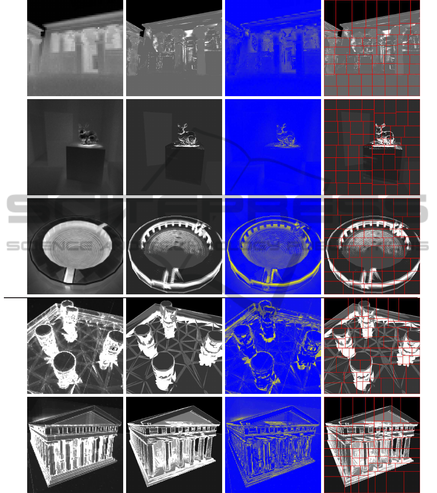
Path tracing
whitted
(a) Real cost map (b) GPU cost map (c) Difference (d) Adaptive tiling
Figure 12: Effectiveness of the cost map generation in different test scenes. For each scene, we show the real packet-based
cost map based on timings (a); the GPU-based cost map estimate (b); an explanatory difference map mapped on a gradient:
In blue areas estimation is precise, whereas yellow areas show less accuracy. (c); the resulting adaptive tiling (d). The cost
maps are obtained mapping the cost of the pixel/packet into the range [0,1].
Even though work stealing is a popular approach
to distributed dynamic load balancing, its perfor-
mance is not well understood yet. The effectiveness
of our sorting-based approach raises new interesting
applications in the context of massively parallel pro-
cessing. In our system, work stealing is particularly
efficient when we have more than 8 workers. Hence,
it seems to be a perfect candidate for today’s and fu-
GPUCostEstimationforLoadBalancinginParallelRayTracing
149

ture massively parallel systems. Our steal analysis
also shows that the number of steal transfers is lower
with high workloads. We suppose that this is related
to the fixed number of tiles size and we plan to inves-
tigate how to beneficially change this number accord-
ing to the workload. Increasing the quality, e.g. using
more samples per pixel and using path tracing, only
slightly affects the scalability of the system.
Scalability. In order to determine how our system
scales with the number of distributed workers, we
ran a scalability test with 1, 4, 8, and 16 workers.
Figure 11 shows the scalability for the Cornell box
test scene. Results indicate that the SAT Sorting ap-
proach provides higher scalability and is particularly
useful with high workloads. The improvement of the
SAT Sorting strategy, compared to a na¨ıve balancing-
unaware approach is about 13-23% with 16 workers.
Efficiency is always superior to 95% with Whitted
style ray tracing test scenes. Instead, using path trac-
ing we have slightly lower performance, with an effi-
ciency of at least 91% with 16 workers.
8 CONCLUSIONS
In this paper, we described a GPU-based algorithm
used to compute a per-pixel ray tracing cost estimate.
The proposed approach, based on deferred shading
and image sampling, is fast and requires only a fixed
amount of GPU memory that increases linearly with
image size and produces a good approximation of the
real computation time. Moreover, our approach could
use any type of cost estimate; for instance it could
also be applied to a cost map produced by using the
ray tracing algorithm itself (i.e. profiling).
In order to validate our idea, we implemented a
parallel ray tracing system for distributed memory
architectures based on Whitted-style ray tracing and
path tracing. Together with our ray tracing system,
we also presented two methods that exploit the cost
map in order to speed up performance: SAT Adaptive
Tiling uses the cost map in order to subdivide the im-
age in tile with the same cost and SAT Sorting instead
exploits the cost map using a dynamic load balanc-
ing, and sorts tiles according to their cost. Our results
indicate that while the SAT Adaptive tiling is more
sensitive to the cost map approximation, SAT Sorting
is always the best approach. It fits well into dynamic
load balancing and provides good scalability for mul-
tiple workers.
In future work, we plan to introduce an automatic
cost map tool to facilitate the tuning of the cost map
generation algorithm. We would like to see how effec-
tive these techniques can be for GPU-based ray trac-
ing implementations (e.g. Nvidia OptiX (Parkeret al.,
2010) employs a three-tiered dynamic load balancing
approach on multi-GPUs). Moreover, we are inter-
ested in evaluating the effectiveness of the techniques
while having models that do not fit the GPU memory,
hence by using a simplification technique for the cost
map computation. With increasingly more computa-
tional power for commodity hardware and the avail-
ability of multicore architectures, we believe that sim-
ilar balancing techniques will become of growing in-
terest in the next future.
ACKNOWLEDGEMENTS
Part of this work was funded by the Austrian Sci-
ence Foundation FWF (DK+CIM, W1227) and also
by the Austrian Ministry of Science BMWF as part of
the UniInfrastrukturprogramm of the Research Plat-
form Scientific Computing at the University of Inns-
bruck.The first author initiated this work at the Visu-
alization Research Center, Universit¨at Stuttgart, and
has been partially funded by a DAAD Scholarship and
a HPC-EUROPA2 project(228398). Carsten Dachs-
bacher acknowledges support from the Intel Visual
Computing Institute, Saarbruecken.
REFERENCES
Baxter, III, W. V., Sud, A., Govindaraju, N. K., and
Manocha, D. (2002). GigaWalk: Interactive Walk-
through of Complex Environments. In Eurographics
workshop on Rendering, EGRW, pages 203–214.
Benthin, C., Wald, I., and Slusallek, P. (2003). A Scalable
Approach to Interactive Global Illumination. Com-
puter Graphics Forum, 22(3):621–630.
Bigler, J., Stephens, A., and Parker, S. (2006). Design for
Parallel Interactive Ray Tracing Systems. In IEEE
Symposium on Interactive Ray Tracing, pages 187 –
196.
Blumofe, R. D. and Leiserson, C. E. (1999). Scheduling
multithreaded computations by work stealing. Journal
of ACM, 46(5):720–748.
Budge, B., Bernardin, T., Stuart, J., Sengupta, S., Joy, K.,
and Owens, J. (2009). Out-of-core Data Management
for Path Tracing on Hybrid Resources. In Eurograph-
ics.
Carpenter, L. (1984). The A-buffer, an antialiased hidden
surface method. In ACM SIGGRAPH, pages 103–108.
Chalmers, A., Debattista, K., Sundstedt, V., Longhurst, P.,
and Gillibrand, R. (2006). Rendering on Demand. In
EGPGV, pages 9–17.
Chalmers, A. and Reinhard, E. (2002). Pratical Parallel
Rendering. AKPeters.
GRAPP2013-InternationalConferenceonComputerGraphicsTheoryandApplications
150

Cosenza, B. (2008). A Survey on Exploiting Grids for Ray
Tracing. In Eurographics Italian Chapter Conference,
pages 89–96.
Cosenza, B., Cordasco, G., De Chiara, R., Erra, U., and
Scarano, V. (2008). Load Balancing in Mesh-like
Computations using Prediction Binary Trees. In Sym-
posium on Parallel and Distributed Computing (IS-
PDC), pages 139–146.
Crow, F. C. (1984). Summed-area Tables for Texture Map-
ping. In 11th annual Conference on Computer Graph-
ics and Interactive Techniques, SIGGRAPH, pages
207–212.
DeMarle, D. E., Gribble, C. P., Boulos, S., and Parker, S. G.
(2005). Memory Sharing for Interactive Ray Tracing
on Clusters. Parallel Comput., 31(2):221–242.
DeMarle, D. E., Gribble, C. P., and Parker, S. G. (2004).
Memory-Savvy Distributed Interactive Ray Tracing.
In EGPGV, pages 93–100.
DeMarle, D. E., Parker, S., Hartner, M., Gribble, C., and
Hansen, C. (2003). Distributed Interactive Ray Trac-
ing for Large Volume Visualization. In IEEE Sym-
posium on Parallel and Large-Data Visualization and
Graphics, PVG, pages 12–.
Dietrich, A., Stephens, A., and Wald, I. (2007). Exploring
a Boeing 777: Ray Tracing Large-Scale CAD Data.
IEEE Comput. Graph. Appl., 27(6):36–46.
Garanzha, K. and Loop, C. T. (2010). Fast Ray Sorting and
Breadth-First Packet Traversal for GPU Ray Tracing.
Computer Graphics Forum, pages 289–298.
Georgiev, I. and Slusallek, P. (2008). RTfact: Generic con-
cepts for flexible and high performance ray tracing. In
Interactive Ray Tracing, 2008. RT 2008. IEEE Sym-
posium on, pages 115 –122.
Gillibrand, R., Longhurst, P., Debattista, K., and Chalmers,
A. (2006). Cost prediction for global illumination us-
ing a fast rasterised scene preview. In AFRIGRAPH,
pages 41–48.
Glassner, A. S. (1989). An Introduction to Ray Tracing.
Morgan Kaufmann.
Grama, A., Karypis, G., Kumar, V., and A., G. (2003). In-
troduction to Parallel Computing, 2nd edition. Pear-
son Addison Wesley.
Hargreaves, S. (2004). Deferred shading. Game Developers
Conference Talks.
Heirich, A. and Arvo, J. (1998). A Competitive Analysis of
Load Balancing Strategies for Parallel Ray Tracing.
Journal of Supercomputing, 12(1-2):57–68.
Hensley, J., Scheuermann, T., Coombe, G., Singh, M., and
Lastra, A. (2005). Fast Summed-Area Table Genera-
tion and its Applications. Computer Graphics Forum,
24(3):547–555.
Ize, T., Brownlee, C., and Hansen, C. D. (2011). Real-Time
Ray Tracer for Visualizing Massive Models on a Clus-
ter. In EGPGV, pages 61–69.
Lauterbach, C., Garland, M., Sengupta, S., Luebke, D., and
Manocha, D. (2009). Fast bvh construction on gpus.
Computer Graphics Forum, pages 375–384.
Moloney, B., Weiskopf, D., M¨oller, T., and Strengert,
M. (2007). Scalable Sort-First Parallel Direct Vol-
ume Rendering with Dynamic Load Balancing. In
Symposium on Parallel Graphics and Visualization
(EGPGV), pages 45–52.
Mueller, C. (1995). The sort-first rendering architecture for
high-performance graphics. In Symposium on Inter-
active 3D graphics, I3D, pages 75–ff.
Muuss, M. J. (1995). Towards real-time ray-tracing of com-
binatorial solid geometric models. In BRL-CAD Sym-
posium.
Odom, C. N., Shetty, N. J., and Reiners, D. (2009). Ray
Traced Virtual Reality. In ISVC, pages 1031–1042.
Overbeck, R., Ramamoorthi, R., and Mark, W. (2008).
Large ray packets for real-time whitted ray tracing. In
Interactive Ray Tracing, 2008. RT 2008. IEEE Sym-
posium on, pages 41 –48.
Parker, S. G., Bigler, J., Dietrich, A., Friedrich, H., Hobe-
rock, J., Luebke, D., McAllister, D., McGuire, M.,
Morley, K., Robison, A., and Stich, M. (2010). Op-
tix: a general purpose ray tracing engine. ACM Trans.
Graph., 29(4):66:1–66:13.
Plachetka, T. (2002). Perfect load balancing for demand-
driven parallel ray tracing. In International Euro-Par
Conference on Parallel Processing, pages 410–419.
Reinhard, E., Kok, A. J. F., and Chalmers, A. (1998). Cost
distribution prediction for parallel ray tracing. In Eu-
rographics Workshop on Parallel Graphics and Visu-
alisation, pages 77–90.
Reshetov, A., Soupikov, A., and Hurley, J. (2005). Multi-
level ray tracing algorithm. In ACM SIGGRAPH,
pages 1176–1185.
Wald, I. (2004). Realtime Ray Tracing and Interactive
Global Illumination. PhD thesis, Computer Graphics
Group, Saarland University.
Wald, I., Dietrich, A., and Slusallek, P. (2004). An Inter-
active Out-of-Core Rendering Framework for Visual-
izing Massively Complex Models. In Eurographics
Symposium on Rendering.
Wald, I., Slusallek, P., Benthin, C., and Wagner, M. (2001).
Interactive Distributed Ray Tracing of Highly Com-
plex Models. In Eurographics Workshop on Render-
ing Techniques, pages 277–288.
Yang, J. C., Hensley, J., Gr¨un, H., and Thibieroz, N. (2010).
Real-Time Concurrent Linked List Construction on
the GPU. Comput. Graph. Forum, 29(4):1297–1304.
Zhou, K., Hou, Q., Wang, R., and Guo, B. (2008). Real-
time KD-tree construction on graphics hardware. In
ACM SIGGRAPH Asia, pages 126:1–126:11.
GPUCostEstimationforLoadBalancinginParallelRayTracing
151
