
Experimental Evaluation of Probabilistic Similarity
for Spoken Term Detection
Shi-wook Lee
1
, Hiroaki Kojima
1
, Kazuyo Tanaka
2
and Yoshiaki Itoh
3
1
National Institute of Advanced Industrial Science and Technology (AIST), Tokyo, Japan
2
Tsukuba University, Tsukuba, Japan
3
Iwate Prefectural University, Takizawa Iwate-gun, Iwate, Japan
Keywords: Speech Recognition, Spoken Term Detection, Probabilistic Similarity, Likelihood Ratio, Gaussian Mixture
Models.
Abstract: In this paper, the use of probabilistic similarity and the likelihood ratio for spoken term detection is
investigated. The object of spoken term detection is to rank retrieved spoken terms according to their
distance from a query. First, we evaluate several probabilistic similarity functions for use as a sophisticated
distance. In particular, we investigate probabilistic similarity for Gaussian mixture models using the closed-
form solutions and pseudo-sampling approximation of Kullback–Leibler divergence. And then we propose
additive scoring factors based on the likelihood ratio of each individual subword. An experimental
evaluation demonstrates that we can achieve an improved detection performance by using probabilistic
similarity functions and applying the likelihood ratio.
1 INTRODUCTION
With the increasing availability of high-speed
networks and gigantic storage devices, the
information sources to which traditional information
science are being applied have expanded explosively
to encompass multimedia, including audio, video,
and graphics, from conventional text-based data
structures. As it has become possible to use large
amounts of multimedia as information, the need for
technologies that allow convenient access to the
multimedia based on content has grown. However,
in order to search multimedia data, data
preprocessing such as manually attaching tag
information when the multimedia is created and
uploaded is unavoidable. One of the most preferred
preprocessing methods for speech-based multimedia
is to use automatic speech recognition (ASR). A
number of studies on content-based retrieval
methods applied to spoken data have been explored
and have achieved remarkable progress over the past
decade. Spoken term detection (STD) is a
fundamental task for speech-based multimedia
information retrieval. The aim of STD is to search
vast, heterogeneous audio archives for occurrences
of specific spoken terms (NIST, 2006). The main
problem with retrieving information from spoken
data is the uncertainty of the automatic transcription.
Especially, any word in speech that is not in the
vocabulary, i.e., out-of-vocabulary (OOV) words,
will be misrecognized as an alternate that has similar
acoustic features. Word-based recognition systems
are usually based on a fixed vocabulary, resulting in
an index with a limited number of words, and so do
not permit searching for OOV words. Even though
such systems can be quickly updated to enroll newly
input words, it is generally difficult to obtain
sufficient data to train the language models that
include OOV words. An alternative method by
which to solve the OOV problem is to use subwords,
such as phonemes, morphemes, and syllables. We
have previously developed a subword speech
recognizer and have proposed new subword units,
i.e., sub-phonetic segments (SPS) (Lee et al., 2005).
In subword recognition, shorter units are more
robust to errors and word variants than longer units,
but longer units capture more discriminative
information and are less susceptible to false matches
during retrieval. In the present paper, to cope with
the uncertainty due to recognition errors, we adopt
soft matching by applying a dynamic programming
approach. In soft matching, the performance of STD
is heavily dependent on the scoring strategy.
441
Lee S., Kojima H., Tanaka K. and Itoh Y. (2013).
Experimental Evaluation of Probabilistic Similarity for Spoken Term Detection.
In Proceedings of the 2nd International Conference on Pattern Recognition Applications and Methods, pages 441-446
DOI: 10.5220/0004264304410446
Copyright
c
SciTePress

2 SCORING IN SPOKEN TERM
DETECTION
The problem is that the inevitable uncertainty of
ASR must be taken into account. When subword
sequences are generated with errors by an ASR, soft
matching like dynamic programming is more
effective for dealing with these errors while
minimizing the number of false term insertions.
2.1 Spoken Term Detection by Shift
Continuous Dynamic Programming
The previously proposed Shift-Continuous Dynamic
Programming (SCDP) is used to detect the input
spoken term as query from the references, which is
the target database (Lee et al., 2005). First, an ASR
encodes database to a linear sequence of subwords.
And then, the SCDP carries out a subword match
between query and database. Finally, the detected
spoken terms are presented in ascending order of
their DP score, given as follows:
,
2,1
3∙
,
3∙
,
1,1
3∙
,
1,2
2∙
,
,
(1)
G(i,r) denotes the cumulative distance up to
reference subword s
r
and input query subword s
i
.
D(·) is local distance, which uses a previously
calculated distance. Here, the straightforward
approach to calculate the distance with errorful
recognition results is to use confusion matrix which
can be readily derived from the training data.
However, estimating the entire confusion matrix is
practically very difficult due to insufficient data.
Furthermore, since the training data confusion
matrix is different from the testing data confusion
matrix, the precise subword confusion matrix is hard
to estimate. From these considerations, we adopt two
scores for calculating the distance in eq. (1). One is
the distance between two probabilistic distributions,
and the other is a measure of the reliability of each
individual subword with respect to the entire
probabilistic feature space.
2.2 Scoring by Probabilistic Similarity
A score is calculated for ranking the retrieved results
that represents the similarity between the detected
part of the utterance and the input query. The
simplest method for measuring the amount of
difference between two sequences is the edit
distance. However, in order to consider inevitable
recognition errors, the score has to quantify the
degree of mutual misrecognition due to similarity
between two probabilistic distributions. For more
sophisticated scoring than the edit distance, the use
of distance between acoustic probabilistic
distributions is very useful. Therefore, in the
proposed method, we calculate distance matrices
from Kullback–Leibler (KL) divergence,
Bhattacharya distance, etc., and then evaluate them
with respect to STD. Such distance matrices give the
degree of the confusion between two subwords.
2.3 Scoring by Likelihood Ratio
In addition to the distance between two subwords,
the recognition performance of each individual
subword should be considered as a score. Since the
uncertainty of speech recognition depends on the
individual subwords, a confidence measure (CM)
using a likelihood ratio (LR) can also be taken as a
score in ranking.
3 PROBABILISTIC SIMILARITY
3.1 Kullback-Leibler(KL) Divergence
KL divergence and its symmetric extension, the
distance, provide objective statistical indicators for
the difficulty in discriminating between two
probabilistic distributions (Kullback and Leibler,
1951) and are widely used tools in statistics and
pattern recognition. Between two distributions f(x)
and g(x), the KL divergence (or relative entropy) is
defined as
||
≡
(2)
For single-mixture multivariate Gaussian
distributions f(x) = N(x;µ
f
,Σ
f
) and g(x) = N(x;
µ
g
,Σ
g
), there is a closed form for KL divergence,
||
1
2
Σ
Σ
Σ
Σ
Σ
d
(3)
where |Σ| denotes the determinant of the matrix, and
Tr(Σ) denotes its trace. Since KL divergence is not
symmetric, it is not a distance metric in the strict
sense. However, we may modify it to make it
ICPRAM2013-InternationalConferenceonPatternRecognitionApplicationsandMethods
442

symmetric. Over the last several years, various
measures to symmetrize the KL divergence have
been introduced in the literature. Among these
measures, we choose simply summing the two
combinations to define KL distance:
,
||
||
(4)
Although Jeffreys (Jeffreys, 1946) do not develop
Eq. (4) to symmetrize KL divergence, the so-called
J-divergence equals the sum of the two possible KL
divergences between a pair of probabilistic
distributions. Because using full covariance causes
the number of parameters to increase in proportion
to the square of dimensions of the features, a
diagonal covariance matrix is generally adopted, in
which the elements outside the diagonal are taken to
be zero. In this case, Gaussian distributions have
independent and uncorrelated dimensions. So Eq. (4)
can be written as the following closed-form
expression:
,
1
2
1
1
2
(5)
3.2 Approximation by the Nearest Pair
In speech recognition, the KL distance is required to
be calculated for GMMs. However, it is not easy to
analytically determine the KL distance between two
GMMs. For GMMs, the KL distance has no closed-
form expression, such as the one shown in Eq. (5).
For this reason, approximation methods have been
introduced for GMMs. The simple method adopted
here is to use the nearest pair of mixture
distributions (Hershey and Olsen, 2007),
,
min
,
,
(6)
where i, j are components of mixture M. As shown
in Eq. (5) and (6), the mixture weight is not
considered at this stage. So this approximation using
a closed-form expression is still based on a single
Gaussian distribution. In our experiments, the
average (d
KL2ave
) and the maximum (d
KL2max
) are also
evaluated.
3.3 Approximation by Montecarlo
Method
In addition to approximation based on the closed-
form expression, the KL distance can be
approximated from pseudo-samples using the Monte
Carlo method. Monte Carlo simulation is the most
suitable method to estimate the KL distance for
high-dimensional GMMs. An expectation of a
function over a mixture distribution,
f(x)=Σπ
m
N(x;µ
m
,σ
2
m
), can be approximated by
drawing samples from f(x) and averaging the values
of the function at those samples. In this case, by
drawing the sample x
1
, …,x
N
~ f(x), we can
approximate (Bishop, 2006).
||
||
≡
1
(7)
In this approximation, Eq. (7), D
MC
(f||g) converges
to D(f||g) as N→∞. To draw x from the GMM f(x),
first, the size of the sample is determined on the
basis of the prior probability of each distribution, π
m
,
and then samples are generated from each single
Gaussian distribution.
3.4 Approximation by Gibbs Sampler
Furthermore, for sampling from multivariate
probabilistic distributions, the Markov Chain Monte
Carlo (MCMC) method has been widely applied to
simulate the desired distribution. A Gibbs sample is
drawn such that it depends only on the previous
variable. The conditional distribution of the current
variable x
f
on the previous variable x
g
has the
following normal distribution.
;
,
1
(8)
where, ρ is the correlation coefficient. Herein, the
full-covariance matrix cannot be calculated due to
the insufficient training data in our experiments;
therefore, we adopt the unique correlation
coefficients from the full training data. The 10,000
(10K) samples from the beginning of the chain, the
so-called burn-in period, are removed. In our
experiments, we generate samples of size 10K and
100K for the MC and MCMC methods. For the
symmetric property, we calculate arithmetic mean
(AM), geometric mean (GM), and harmonic mean
(HM) from the resulting KL divergence with MC
and MCMC sampling (Johnson and Sinanovi´c, S.,
2001). The maximum and minimum between the
two divergences, D(f||g) and D(g||f) are also
calculated for comparison.
3.5 Bhattacharyya Distance and Others
The Bhattacharyya distance, which is another
ExperimentalEvaluationofProbabilisticSimilarityforSpokenTermDetection
443

measure of the probabilistic similarity between
GMMs, is also evaluated (Fukunaga, 1990). In the
same way as in approximation by the nearest pair,
first distance between two distributions among the
mixture distributions is computed using the closed-
form of Eq. (9) and then the minimum value is
selected.
,
1
4
1
2
/2
(9)
,
min
,
,
(10)
Here, the average (d
Bave
) and the maximum (d
Bmax
)
are also used for evaluation in the experiments.
Another basic class of distance functions is edit
distances (d
Edit
), in which distance is defined as the
cost of the retrieved term of the edit operation.
Typical edit operations are subword insertion,
deletion, and substitution, and each such operation
much be assigned a cost.
The following distance, Eq. (11), which is
defined for clustering in Hidden Markov Model
Toolkit (HTK) (Young et al., 2009), is also
compared in the experiment. This distance (d
HTK
) is
the average of log-probabilities of the means in the
other distribution. Unlike the other distances so far,
the greater the value, the more similar the two
distributions f and g are. Thus, the ranking order is
reversed.
,
1
log
log
(11)
4 SCORING BY CONFIDENCE
MEASURE
In speech recognition, CMs are used to measure the
uncertainty of recognition results (Jiang, 2005). In
our STD system, the CM calculated on GMMs is
adopted as the score in the ranking. The likelihoods
of all frames in training the acoustic model are
calculated for all GMMs. Then, the likelihood from
the GMM which is labeled by forced alignment and
the maximum likelihood from among all GMMs are
rated to extract a LR. The LR of observed vector o
t
at frame t is defined as follows using the output
probability of GMM, and then all LR from the
training frames (T) are averaged for each GMM as a
CM.
1
1
(12)
Here b
max
is the output probability of the GMM with
the maximum likelihood from among all GMMs,
and b
FA
is the output probability of the labeled
GMM that is generated from the forced alignment. If
b
FA
= b
max
, LR(o
t
) is equal to one. In the
experiments, the likelihoods are calculated from
1389 GMMs, consisting of 463 SPSs in Japanese.
The weighted α(1 - CM) which is estimated from Eq.
(12) is added to the Bhattacharyya distance of Eq.
(10), and the resulting score is used to rank the
retrieved term.
1
,′
1
(13)
where, W is the total number of GMMs in the query.
The CM appearing in Eq. (13) is one of the
following types: 1) likelihood ratio given in Eq.
(11), calculated from all the training data (LRall), 2)
log odds of a likelihood ratio (log odds of LRall ; log
(odds) = log (prob. / (1-prob)) ), 3) likelihood ratio
calculated from the frames in which only the GMM
of the forced alignment label does not have
maximum likelihood (LRincorr), and 4) the correct
rate (Corr), for comparison. The correct rate is a
direct measure of how well SPS can be recognized
correctly.
5 EXPERIMENTAL
EVALUATION
5.1 Japanese Spoken Term Detection
Task
In this section, we present experimental results for
Japanese open-vocabulary spoken term detection.
The corpus consisted of 10 news paragraphs in
Japanese, read 30 times by 19 speakers (13 men and
6 women). Thus, the corpus is composed of 300
paragraphs. Each paragraph is approximately one
minute long, and the total length of the corpus is 377
minutes (6 hours and 17 minutes). Each paragraph
contains 10 keywords, which are each uttered twice.
Thus each keyword has 60 relevant locations in the
entire corpus. Our task is to detect when the spoken
term is uttered for a given text query. In Japanese,
text can be converted into its phonetic representation
using conversion rules, whether the query term is
ICPRAM2013-InternationalConferenceonPatternRecognitionApplicationsandMethods
444

OOV or in-vocabulary. To calculate the CM and
train the GMM of SPSs, 187 hours speech of the
Corpus of Spontaneous Japanese (CSJ) database, are
used (Maekawa, 2003). Each GMM-based acoustic
model is a 38-dimension (12-MFCC, 12-ΔMFCC,
12-ΔΔMFCC, 1-ΔPOWER, 1-ΔΔPOWER) and 8-
mixture Hidden Markov Model.
For evaluating performance, we use precision
and recall with respect to manual transcription. Let
Correct(q,j) be the number of times that query q is
retrieved correctly in the j-th ranked document. Let
Retrieved(q) be the number of retrieved documents
for query q, and let Relevant(q) be the total number
of times that q appears in the database.
,
,
(14)
,
,
(15)
We compute the precision and recall rates for each
query, and then summarize them into the F-measure,
which is defined as
2
(16)
The maximum F-measure of each query is presented
in order to summarize the information in a precision
-recall curve as a single value. We average the maxi
mum F-measure over all queries and then multiply it
by 100 to give it as a percentage, referred to this as
Ave. of Max. F-measure.
5.2 Experimental Results
As shown in Table 1, using sophisticated score of
the similarity between probabilistic distributions is
effective in STD. Comparing d
Bmin
to the result with
the edit distance(d
edit
), the spoken term detection
performance is significantly increased from 88.21 up
to 94.02. It can be confirmed that using probabilistic
similarity can take into account the uncertainty of
ASR. Also, the use of KL divergence as distance is
effective to detect spoken term with errors. From
these experimental results, the sophisticated score of
probabilistic similarity can be implemented to
improve the spoken term detection. In Bhattacharyya
distance and Kullback-Leibler distance, using the
distance calculated from the nearest pair (d
Bmin
and
d
KL2min
) is more effective than the use of the distance
from the farthest pair of the mixture components
(d
Bmax
and d
KL2max
) and the average (d
Bave
and d
KL2ave
)
between all mixture components. It can be proved
that the recognition error between two GMMs has
mostly occurred in the nearest pair.
Table 1: Experimental results of using edit distance and
approximate distances based on closed-form expression.
Ave. of Max. F-measure
d
edit
88.21
d
Bmin
94.02
d
Bave
91.99
d
Bmax
87.98
d
KL2min
93.95
d
KL2ave
90.55
d
KL2max
82.27
d
HTK
91.71
As shown in Table 2, the distance approximated by
pseudo-samples is also effective for scoring in STD.
Since the multi-variant feature vectors used in
speech recognition are mutually correlated, even
though diagonal covariance matrices are used for
computational convenience, using MCMC is better
than the simple MC. For the symmetric metric, using
the minimum value has better performance than any
of the average methods (AM, GM, or HM) and using
the maximum value.
Table 2: Experimental results of using approximate
distances by pseudo-samples (MC and MCMC).
MC
# of
samples
Ave. of Max. F-measure
AM GM HM
100K 91.50 91.51 91.49
10K 91.51 91.51 91.49
min max
100K
91.59 91.28
MCMC
(Gibbs)
AM GM HM
100K
92.07 92.02 92.05
10K 92.08 92.02 92.05
min max
100K
92.17 91.87
Since the correlation coefficients in the MCMC
approach are uniquely obtained from the entire
training data set, the values are slightly less accurate.
However, the experiments do confirm the
effectiveness of the MCMC method. In future work,
we will try to draw the pseudo-samples using exact
correlation coefficients.
The experiments are performed by adding
weighted CM of the discussed four types to the
Bhattacharyya distance (d
Bmin
) and the edit distance
(d
Edit
). As shown in Figs. 1 and 2, improved
ExperimentalEvaluationofProbabilisticSimilarityforSpokenTermDetection
445
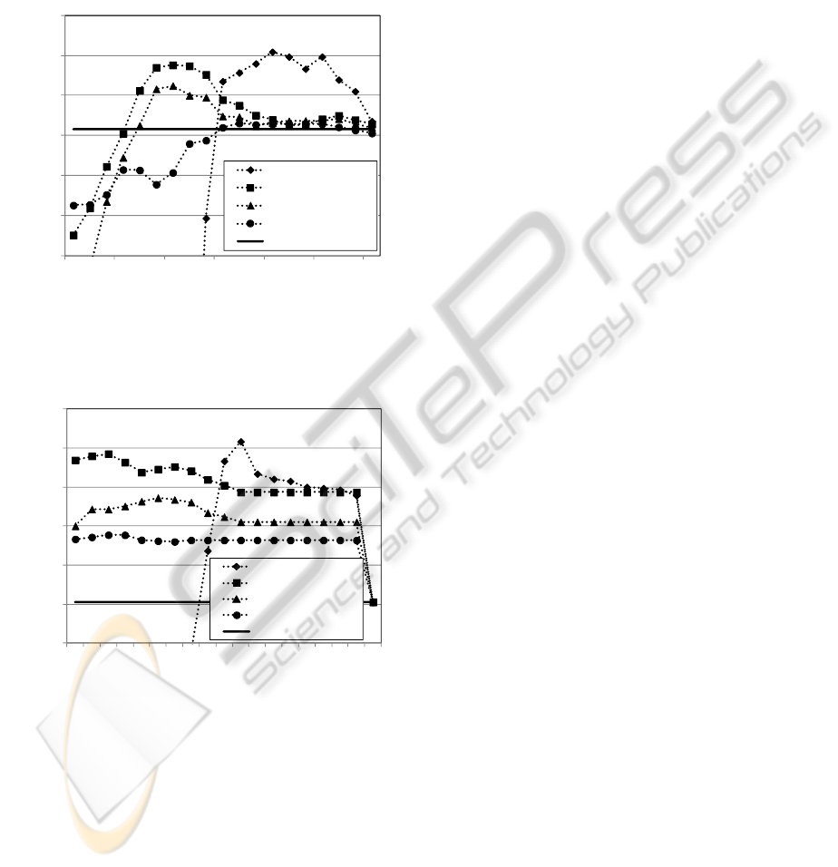
performance can be achieved by adding the CM of
subwords to distances. From the experimental results,
we can confirm that the distance from probabilistic
similarity can be used to measure the amount of
misrecognition between subwords and the likelihood
ratio can be used to evaluate the uncertainty of the
subword itself.
Figure 1: Retrieval performance (Ave. of max. F-measure)
based on the minimum(=nearest pair) of Bhattacharyya
distance, d
Bmin
and adding weighted CM.
Figure 2: Retrieval performance (Ave. of max. F-measure)
based on edit distance, d
edit
and adding weighted CM.
6 CONCLUSIONS
In this paper, the use of the probabilistic similarity
and likelihood ratio for spoken term detection was
investigated, and different ways of evaluating the
probabilistic similarity is compared and tested. First,
we compare several types of probabilistic similarity
measures. The symmetric Kullback-Leibler distance
and Bhattacharyya distance are effective distance
metrics to facilitate spoken term detection. Then, we
proposed an additive score that takes into account
confidence. From the experimental results, the
improved performance in Spoken Term Detection
confirms the efficiency of the proposed sophisticated
scoring strategy.
REFERENCES
NIST, 2006. The Spoken Term Detection (STD) 2006
Evaluation Plan. From http://www.nist.gov/speech/
tests/std/docs/std06-evalplan-v10.pdf.
Lee, S. W., Tanaka, K. and Itoh, Y., 2005. “Combining
Multiple Subword Representations for Open-
vocabulary Spoken Document Retrieval”, In
ICASSP’05, pp. 505-508.
Kullback, S. and Leibler, R. A., 1951. “On Information
and Sufficiency”, In The Annals of Mathematical
Statistics, Vol. 22, No. 1, pp.79-86.
Jeffreys, H., 1946. “An invariant form for the prior
probability in estimation problem”, In Proceedings of
the Royal Society of London. Series A, Mathematical
and Physical Sciences Vol. 186, No. 1007, pp. 453-461.
Hershey, J. R. and Olsen, P. A., 2007. “Approximating the
Kullback Leibler Divergence between Gaussian
Mixture Models”, In Proceedings of IEEE
International Conference on Acoustics, Speech and
Signal Processing, pp.317-320.
Bishop, C. M., 2006. “Pattern Recognition and Machine
Learning”, Springer, pp.55-58, pp.85-87.
Johnson, D. H. and Sinanovi´c, S., 2001. “Symmetrizing
the Kullback-Leibler distance,” In IEEE Trans. on
Information Theory.
Fukunaga, K., 1990. “Introduction to Statistical Pattern
Recognition”, second ed., New York: Academic Press.
Young, S., Evermann, G., et al., 2009. “The HTK Book
(for HTK Version 3.4)”.
Jiang, H., 2005. “Confidence Measures for Speech
Recognition: A Survey”, In Speech Communication,
Vol. 45, pp. 455-470.
Maekawa, K., 2003. “Corpus of Spontaneous Japanese: Its
Design and Evaluation”, In Proceedings of the ISCA &
IEEE Workshop on Spontaneous Speech Processing
and Recognition (SSPR2003).
94.21
94.17
94.12
94.03
94.02
93.7
93.8
93.9
94.0
94.1
94.2
94.3
0.100 0.070 0.040 0.010 0.007 0.004 0.001
Ave. of max. F-measure
weight(α)
+ log odds of LR all
+ LR al
l
+ Corr
+ LR incorr
d
Bmin
(Baseline)
89.03
88.97
88.74
88.55
88.21
88.0
88.2
88.4
88.6
88.8
89.0
89.2
1.20 0.90 0.60 0.30 0.09 0.06 0.00
Ave. of max. F-measure
weight(α)
+ log odds of LR all
+ LR all
+ Corr
+ LR incorr
d
edit
(Baseline)
ICPRAM2013-InternationalConferenceonPatternRecognitionApplicationsandMethods
446
