Cluster Detection and Field-of-View Quality Rating

Applied to Automated Pap-smear Analysis

Marine Astruc

, Patrik Malm

, Rajesh Kumar

and Ewert Bengtsson

Ecole Centrale Nantes, Nantes, France

Centre for Image Analysis, Division of Visual Information and Interaction, Department of Information Technology,

Uppsala University, Uppsala, Sweden

Centre for Development of Advanced Computing, Thiruvananthapuram, India

Keywords:

Pap-smear, Automated Screening, Cluster Detection, Field-of-View Analysis.

Abstract:

Automated cervical cancer screening systems require high resolution analysis of a large number of epithelial

cells, involving complex algorithms, mainly analysing the shape and texture of cell nuclei. This can be a very

time consuming process. An initial selection of relevant ﬁelds-of-view in low resolution images could limit

the number of ﬁelds to be further analysed at a high resolution. In particular, the detection of cell clusters

is of interest for nuclei segmentation improvement, and for diagnostic purpose, malignant and endometrial

cells being more prone to stick together in clusters than other cells. In this paper, we propose methods aiming

at evaluating the quality of ﬁelds-of-view in bright-ﬁeld microscope images of cervical cells. The approach

consists of the construction of neighbourhood graphs using the nuclei as the set of vertices. Transformations

are then applied to such graphs in order to highlight the main structures in the image. The methods result in

the delineation of regions with varying cell density and the identiﬁcation of cell clusters. Clustering methods

are evaluated using a dataset of manually delineated clusters and compared to a related work.

1 INTRODUCTION

According to the World Health Organization (WHO)

cervical cancer is the second most common type

of cancer among women, annually killing close to

300,000 world wide. Out of these deaths 86% oc-

cur in developing countries (WHO/ICO Information

Centre on HPV and Cervical Cancer (HPV Informa-

tion Centre), 2012). An important reason to the large

difference is the absence of organized screening pro-

grammes using the Papanicolaou test (Pap test) de-

veloped by Dr. Georges Papanicolaou in the 1940s

(Papanicolaou et al., 1943). For this test cells are ob-

tained from the uterine cervix through a simple scrap-

ing/brushing operation and smeared onto a glass slide

of 25x75 mm, ﬁxated and stained and then inspected

through a normal light microscope at high resolution.

Based on a Pap-test, trained cytologists can not

only ﬁnd proof of invasive cancer but also detect cer-

tain cancer precursors, allowing for early and effec-

tive treatment. If detected early, invasive cancer is

curable and the 5-year survival rate as high as 92%

(Saslow et al., 2012).

Most screening programmes revolve around vi-

sual screening performed by cytotechnicians in spe-

cialized laboratories. The screening work is tedious

and, often due to fatigue, error prone. Because of the

hazards of fatigue some recommendations say that a

cytotechnician should not work more than 7 hours a

day and analyse no more than 70 samples (Elsheikh

et al., 2012). This implies an average time to analyze

a specimen of 6 minutes, a very short time given the

complexity of the task.

Although the Pap test has shown its worth through

decades of use it is hampered by a number of difﬁcul-

ties, e.g., variable smear thickness, uneven cell distri-

bution, dense cell groupings (clusters), obscuring ele-

ments such as blood and inﬂammatory cells and vari-

able ﬁxation and staining results (Grohs and Husain,

1994).

To overcome some of the human limitations sev-

eral attempts to automate the screening process have

been made since the 1950s with varying degree of

success. Today there are systems that are able to per-

form a scan of a sample but they all have in common

that they require very speciﬁc sample preparation and

are complicated and expensive to run (Bengtsson,

2005).

355

Astruc M., Malm P., Kumar R. and Bengtsson E. (2013).

Cluster Detection and Field-of-View Quality Rating - Applied to Automated Pap-smear Analysis.

In Proceedings of the 2nd International Conference on Pattern Recognition Applications and Methods, pages 355-364

DOI: 10.5220/0004254803550364

 SciTePress

A fundamental problem in developing a screening

system is the vast areas that need to be analysed. A

regular PAP-smear covers an area of at least 25x50

mm. The resolution needed for determining the ma-

lignancy of a cell leads to a pixel size of around 0,2

microns. This translates to 31 billion pixels on a spec-

imen. Handling this amount of data in a few minutes

poses serious challenges both on the initial scanning

side and on the subsequent data analysis side. One

way of improving the situation is to use a modiﬁed

technique for depositing the slides on the specimen.

So called Liquid Based Preparations, LBP, typically

deposit the material in a circle with a diameter of 20

mm. This reduces the number of pixels to around 8

billion, still a substantial number, at the cost of a sub-

stantially more complex and costly slide preparation

procedure. For the ﬁnal analysis of a cell to be reliable

it has to be in perfect focus and the algorithms to ex-

tract the relevant features are typically quite elaborate

and thus time consuming. Autofocus and complex

analysis algorithms thus make the automated screen-

ing problem even more challenging.

One way to attack this difﬁculty is to have a two

stage approach, an initial search phase for areas or

cells of interest followed by a detailed analysis of

the interesting regions. This approach was ﬁrst sug-

gested and analyzed by Poulsen (Poulsen, 1973) and

later implemented in the Diascan system (Nordin,

1989). There have been huge improvements in scan-

ning and computer technology since the 1970-80 ies

when these projects were conducted but the funda-

mental problem holds. We thus need to ﬁnd efﬁcient

ways of determining where on the slide we should fo-

cus our attention to reach a reliable decision about

whether the specimen is normal or possibly show

some abnormalities.

The initial analysis can be conducted of ﬁelds of

view of lower resolution and with less stringent re-

quirement on perfect focus. Whether these ﬁelds are

obtained by merging pixels or subsampling images

scanned at full resolution or by a separate scan of

the specimen with different optics is a technical is-

sue that requires a complicated technical/economical

analysis to ﬁnd the best solution for a particular set-

ting. We will not discuss those issues further in this

paper. For the study in this paper we have worked

with images with a pixel size of 0.5 microns and with

a single rough focus setting. This represents between

one and two orders of magnitude less data than the

perfectly focused, high resolution images needed for

the ﬁnal analysis.

The task of this low resolution analysis is to ﬁnd

areas that should be analysed more in detail. This

will trivially mean to discard completely empty ar-

eas or areas where the cells are spread so dense that

they cannot be resolved. We will be looking for areas

with suitable density of cells of potential diagnostic

interest. This could be extended to only look for cells

that are larger than normal, since malignant cells usu-

ally are larger than normal ones. But stretching this

criterion too far risks leading to missing some spec-

imens where the malignant cells are of normal size

(such malignancies exists). So we will be counting

cells that are of a relevant size for further analysis,

not only cells signiﬁcantly bigger than normal.

Another important task is to look for clusters. It is

known that malignant cells tend to cluster more than

normal ones so when the human screener see a clus-

ter of cells they take an extra look. We should thus

note and ﬂag the appearance of clusters in the anal-

ysed ﬁelds.

So to summarize we will in this paper present

a study of image ﬁelds of moderate resolution from

standard PAP smears and LBP specimens generating

data that can be used to prioritize which areas should

be used for the subsequent more expensive high reso-

lution analysis. Thus optimizing the overall through-

put of a system without sacriﬁcing detection qual-

ity. The methods described in this paper can also

work towards the overall classiﬁcation task by locat-

ing diagnostically important structures that are often

overlooked in conventional cell by cell classiﬁcation

schemes. We have not found any studies in the re-

cent literature with this goal, most papers on PAP-

smear analysis deal with segmentation or classiﬁca-

tion problems of images at a single resolution level.

However, Raymond et al. (Raymond et al., 1993)

made use of graphs and mathematical morphology

to analyse neighbourhood relationship between cells

in the study of germinal centers. Also, in a recent

publication Chandran et. al (Chandran et al., 2012)

presented a method for detecting clusters in cervical

smears that is of interest and that is used for compari-

son in this paper.

2 MATERIALS AND METHODS

2.1 Microscope Setup

The images were acquired using an Olympus BX51

optical microscope with a 20X, 0.75 NA objective and

a Hamamatsu ORCA 05G monochrome digital cam-

era providing images of 1344 x 1024 with an effective

square pixel size of 0.5 microns. The illumination was

ﬁltered through a narrow green ﬁlter centered at 570

nm in order to optimize nuclear contrast.

ICPRAM2013-InternationalConferenceonPatternRecognitionApplicationsandMethods

356

2.2 Methodology

The methods developed to analyse an image ﬁeld

from a cervical smear sample are based on transfor-

mations applied to graphs that are built using the cell

nuclei as vertices. The ﬁrst step consists of the seg-

mentation of the cell nuclei. Then, neighbourhood

graphs are constructed and several transformations

are applied to the different graphs in order to separate

the image ﬁeld into three regions according to how

densely the nuclei are spaced and to locate the cells

belonging to clusters.

2.3 Nuclei Segmentation

In order to build graphs on an image ﬁeld, we need to

segment the cell nuclei. A preprocessing step is used

to reduce the background noise and improve the im-

age quality. It consists of the implementation of a me-

dian ﬁlter. The contrast of the grayscale image is en-

hanced using Contrast-Limited Adaptive Histogram

Equalization (Zuiderveld, 1994). As a ﬁrst stage of

the segmentation, grayscale morphological closings

with annular ﬂat structuring elements are applied to

identify nuclei-like objects, which will serve as seeds.

The nuclear boundaries are then delineated using

seeded watershed segmentation (Moshavegh et al.,

2012).

The resulting segmented nuclei-like objects are

then classiﬁed into two groups, nuclei and artifacts,

using Support Vector Machine. To evaluate the classi-

ﬁcation results, a Graphical User Interface (GUI) was

developed to permit a user to identify nuclei in a set of

images. A total of 24 images, belonging to different

samples, have been marked. 2478 objects were man-

ually identiﬁed as nuclei and 5474 identiﬁed as arti-

facts. The sensitivity, the speciﬁcity and the accuracy

of the classiﬁcation are 96,6%, 86,0% and 89,3% re-

spectively. Although the results of segmentation and

classiﬁcation present some errors (missing nuclei, re-

maining artifacts), the objects identiﬁed as nuclei af-

ter the classiﬁcation will be considered as true nuclei

throughout the analysis. These imperfections affect

the results obtained by the methods herein presented.

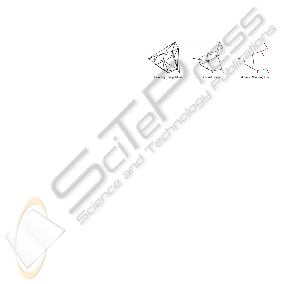
2.4 Graph Generation

After the segmentation of the cell nuclei, we have the

vertex set on which we build neighbourhood graphs.

Formally, a graph G = (V, E) is deﬁned as a set V of

vertices of the graph and a set E of edges of the graph.

The methods developed uses the Voronoi diagram and

neighbourhood graphs stemming from the Voronoi

diagram: the Delaunay triangulation (DT), Gabriel

graph (GG) and the euclidean minimum spanning

tree (MST). Neighbourhood graphs are used in image

analysis to model geometric structures and connect-

edness. The edges deﬁne the neighbourhood relation

”is connected to” on the set of vertices. According

to Vincent (Vincent, 1989), and to Heijmans and Vin-

cent (Heijmans H., 1992), MST, GG and DT are very

interesting for studying proximity problems because

they are connected, unique (except for MST), they do

not depend on any parameter (e.g. a maximal distance

between objects or a minimal number of neighbours)

which implies that they are independent of scaling and

they are included into one another MST ⊆ GG ⊆ DT

[ﬁg. 1], enabling a modelling of neighbourhood rela-

tionships of increasing strength.

Figure 1: Three neighbourhood graphs related to the

Voronoi diagram.

3 GLOBAL ANALYSIS - IMAGE

FIELD SCORE

In order to facilitate the subsequent high resolution

processing of the images we wish to detect regions

with low, medium and high density of cell nuclei. To

achieve this, a global analysis was performed to sepa-

rate the image ﬁeld according to cell density.

• Low density regions: Some regions in the image

ﬁeld are empty or contain very few nuclei.

• Medium density regions: These regions contain

many nuclei distributed quite evenly and belong-

ing mostly to free-lying cells. These are the re-

gions of biggest interest and they should be further

studied, the numerous nuclei allowing to build a

large database of features and measurements.

• High density regions: These regions contain a

very large number of nuclei or artifacts. Most of

the cells are overlapping and closely gathered in

clusters, some are folded and the dense regions

are more prone to be partly out of focus. The

nuclei can be deformed or barely visible. Their

segmentation can be very difﬁcult, leading to use-

less measurements. Hence, special care should be

taken when studying these regions and thus it is

important to identify them.

ClusterDetectionandField-of-ViewQualityRating-AppliedtoAutomatedPap-smearAnalysis

357

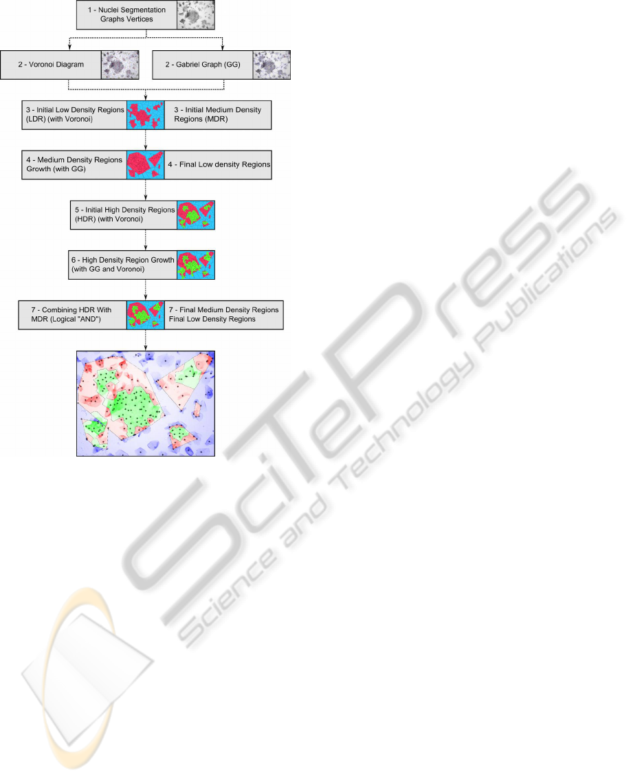
Figure 2: Global analysis method main steps.

The Global Analysis method uses both the Voronoi

Diagram and Gabriel Graph. The main steps of the

method are given in ﬁgure 2. Each step is further

discussed in the following sections. Throughout the

global analysis method, the parameters tuned (such as

thresholds) are normalized by the diameter of the im-

age, in order for the code to be adaptable to any image

size. All the parameters have been set by changing

values experimentally.

3.1 Determining the Low Density

Regions

Low density regions are deﬁned as containing no or

few nuclei. Consequently, these regions hold very

few, spaced out, vertices, and are thus paved by large

Voronoi cells. In order to determine low density re-

gions, the cells in the Voronoi diagram were thresh-

olded according to their area. Each cell in the Voronoi

diagram with an area superior to a threshold is con-

sidered as belonging to a low density region. The rest

of the Voronoi cells are considered as belonging to

medium (or high) density regions [ﬁg. 3 (a)].

3.2 Medium Density Regions Growth

After step 3 [ﬁg. 2], we can observe on the Gabriel

graph that some vertices within the initial low density

regions are close (Euclidean distance) neighbours of

vertices situated inside the medium density regions.

These nuclei should thus be included in the medium

density regions, resulting in larger medium density re-

gion. This operation is repeated as long as vertices

are added. Once all the close-by vertices have been

added to the regions, we apply the convex hull on

each of the grown set of vertices, and thus obtain the

ﬁnal medium density regions. The result is stored in a

binary image, where medium density regions are as-

signed the value 1 and low density regions (the rest of

the image) are assigned the value 0. The contours in

this binary image represent the external contours of

the ﬁnal medium density regions. The internal con-

tours of the medium density regions will be the exter-

nal contours of the high density regions [ﬁg. 3 (b)].

3.3 Initial High Density Regions

High density regions are deﬁned as containing many

closely located nuclei. They are thus paved by small

Voronoi cells. In order to determine high density re-

gions, the cells in the Voronoi diagram were thresh-

olded according to their area. Each cell in the Voronoi

diagram with an area less than a threshold is consid-

ered as belonging to a high density region [ﬁg. 3 (c)].

3.4 High Density Regions Growth and

Final Borders of

the High Density Regions

Likewise step 4 [ﬁg. 2], after step 5, we can observe

on the Gabriel graph that some vertices outside the

initial high density regions are close (Euclidean dis-

tance) neighbours of vertices situated inside the high

density regions. These vertices are added to the high

density regions, but contrary to step 2, the operation is

just executed once, to avoid a too large growth of the

high density regions. Indeed, it was observed experi-

mentally that further iterations would result in adding

irrelevant vertices. Once these nearby vertices have

been added, one can notice that farther vertices be-

longing to high density regions are still considered

as belonging to medium density regions. To solve

this problem, we take into account the grey value of

the Voronoi cells situated in the neighbourhood of the

high density regions, from which we removed the nu-

clei that generated the Voronoi cell. If the mean grey

ICPRAM2013-InternationalConferenceonPatternRecognitionApplicationsandMethods

358

value is inferior to a threshold (dark Voronoi cell), or

if the standard deviation of the grey value is superior

to a threshold with a mean grey-value still quite low

(Voronoi cell with a dark part and a part of higher

intensity, often found at the border of a high density

region), the vertex that generated this Voronoi cell is

added to the high density regions vertices, resulting in

larger high density regions. This operation is repeated

as long as vertices are added. Indeed, high density re-

gions are often very dark due to the closeness of cells,

which justiﬁes taking grey-value into account [ﬁg. 3

(d)].

Once this step has been accomplished, we obtain

n sets of vertices belonging to the grown high density

regions. We extract the Voronoi cells generated by

these vertices, and store them in a binary image with

value 1. Value 0 is assigned to the rest of the image.

This binary image and the medium density regions bi-

nary image mentioned above are combined using the

logical operation AND [ﬁg. 3 (e)]. The binary im-

age thus obtained is the ﬁnal high density binary im-

age, where regions with value 1 represent high den-

sity regions. Indeed, high density regions should be

included in the regions that had previously been iden-

tiﬁed as medium dense, and not encroach upon low

density regions. The contours in this binary image

represent the contour of the ﬁnal high density regions

[ﬁg. 3 (f)].

3.5 Overview of the Results of

the Global Analysis

Figure 4 shows the results obtained with the global

analysis method, for a set of 30 images, 10 images

with mostly high density regions (HDR), 10 images

with mostly medium density regions (MDR) and 10

images with mostly low density regions (LDR).

Four ratios are calculated:

Ratio 1: Proportion of nuclei in MDR and nuclei in

LDR compared to nuclei in HDR.

nuclei in MDR + nuclei in LDR

nuclei in HDR + 1

(1)

Ratio 2: Proportion of MDR area compared to LDR

and HDR areas.

MDR Area

LDR Area + HDR Area

(2)

Ratio 3: Proportion of HDR area compared to LDR

and MDR areas.

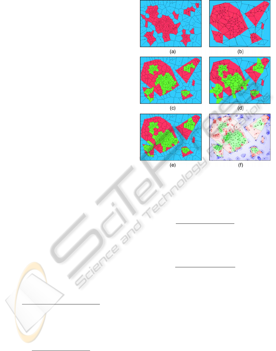
Figure 3: Illustration of the Global Analysis main steps. (a)

Initial low density regions (LDR) (blue) and initial medium

density regions (MDR) (red). (b) Medium density regions

growth and ﬁnal low density regions. (c) Initial high density

regions (HDR) (green). (d) High density regions growth.

(e) Combining HDR and initial MDR. (f) Final regions.

HDR Area

LDR Area + HDR Area

(3)

Ratio 4: Proportion of LDR area compared to HDR

and MDR areas.

LDR Area

HDR Area + MDR Area

(4)

The values obtained for the different ratios differ

according to the density of the nuclei in the image.

Ratio 1 increases when the nuclei density decreases.

For ratio 2 the proportion of MDR area compared to

LDR and HDR areas is much higher for medium den-

sity images than for low or high density images. Like-

wise, for ratio 3, the proportion of HDR area com-

pared to LDR and MDR areas is much higher for high

density images than for low or high density images,

and for ratio 4, the proportion of LDR area compared

to HDR and MDR areas is much higher for low den-

sity images than for medium or high density images.

ClusterDetectionandField-of-ViewQualityRating-AppliedtoAutomatedPap-smearAnalysis

359

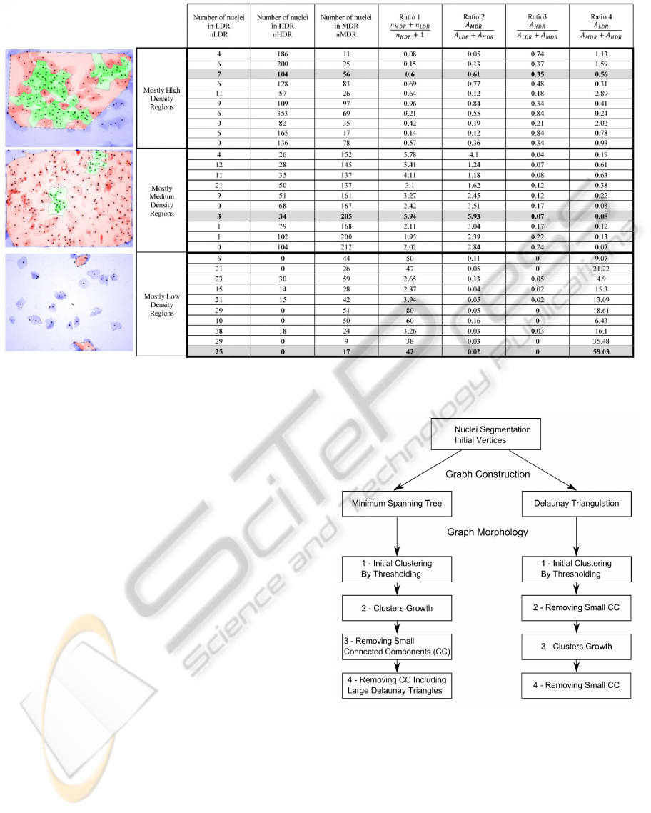
Figure 4: Overview of the results of the global analysis. The ratios values of the displayed images are highlighted.

4 DETECTING CELL CLUSTERS

USING GRAPHS

Cervical cell images usually contain single cells, clus-

ters of cells as well as artifacts. It is important to de-

ﬁne the regions containing cells, clusters of cells, or

regions void of cells in order to reduce the area to be

studied. The detection of cell clusters in an image is

of interest for two reasons. First, cells have different

features when in a cluster, their nuclei can be over-

lapping or out of focus, resulting in the impossibility

to detect or to segment them properly. Special analy-

sis should be applied when studying cells in a cluster,

and therefore it is important to identify the position

of these clusters in the images. Secondly, the pres-

ence of cell clusters in the slide has a diagnostic value,

because malignant cells are more prone to stick to-

gether in clusters than normal cells. Thirdly, endome-

trial cells, which also should be detected, usually form

clusters. Graph theory is known for its ability to anal-

yse complex interactions and relationships in diverse

systems. Vertices correspond to the objects in the sys-

tem and the edges describe the neighbouring relations

between these objects. We have therefore used graph

theoretical methods to detect clusters. Throughout

the clustering method, the parameters tuned (such as

thresholds) are normalized by the diameter of the im-

age, in order for the code to be adaptable to any image

Figure 5: Proposed clustering methods main steps.

size. All the parameters have been set by changing

values experimentally.

4.1 Clustering the Euclidean Minimum

Spanning Tree

Two alternative approaches were tested to analyse the

clusters, which main steps are given in ﬁgure 5. The

ﬁrst method was based on clustering the Euclidean

ICPRAM2013-InternationalConferenceonPatternRecognitionApplicationsandMethods

360

Minimum Spanning Tree (EMST).

4.1.1 Initial Clustering by Thresholding of the

Euclidean Minimum Spanning Tree

In order to obtain initial clusters, the edges in the

EMST are thresholded. Indeed, one feature character-

ising clusters in the EMST is their short edges. Each

edge in the EMST with a length superior to a thresh-

old t

Edges

is removed from the graph. The graph re-

sulting from the thresholding of the EMST is a forest

and the N

different connected components thus ob-

tained represent N

initial clusters.

4.1.2 Cluster Growth

From the previous step, we have obtained N

initial

clusters. The purpose of this step is to make each clus-

ter grow, by adding neighbouring edges similar (in

terms of length) to the edges already present in the ini-

tial cluster. A neighbouring edge is added if its length

divided by the average length of the edges in the initial

cluster is inferior to a threshold t

Edges−growth

. Once

every neighbouring edge has been visited, and pos-

sibly added, the resulting cluster is larger. Then the

operation is repeated on the resulting grown cluster,

as long as neighbouring vertices are added.

Once this step has been accomplished for each ini-

tial cluster that had been obtained after thresholding

of the EMST, we obtain N

clusters CG(grown clus-

ters). Edges and vertices have been added, and some

clusters CG are actually connected in the EMST. They

are then merged in order to identify each connected

components that will form our ﬁnal set of clusters.

We end up with a number of clusters N

≤ N

4.1.3 Removal of Small Connected Components

Connected components containing few vertices are

most of the time ”false clusters”, free-lying cells close

enough from each other to be mistaken as a cluster.

The clusters containing less than a threshold t

Comp

vertices are removed.

4.1.4 Removal of Connected Components

Including Large Delaunay Triangles

Clusters of cells are constituted of several cells very

close to each other (most of the time overlapping),

thus vertices (or nuclei) in clusters are also close to

each other and the Delaunay Triangles made up of

these vertices have a small area. As a result, con-

nected components that include Delaunay triangles of

large area are removed from the clusters list.

The result of the detection of clusters with the

EMST is shown for two cytology images in ﬁgure 6.

Figure 6: Detection of clusters using Euclidean Minimum

Spanning Tree. Black contours represent the clusters as de-

lineated for ground truth.

4.2 Clustering with the Delaunay

Triangulation

The second cluster analysis method was based on

clustering with the Delaunay triangulation (DT).

4.2.1 Initial Clustering by Thresholding of the

Delaunay Triangulation

In order to obtain initial clusters, the triangles in the

Delaunay triangulation were thresholded relatively to

their area and perimeter. Indeed, as noted previously,

vertices in clusters are close to each other, thus the

Delaunay triangles made up on these vertices have

small area and perimeter. Consequently, each trian-

gle in the Delaunay triangulation with an area supe-

rior to a threshold t

Area

and a perimeter superior to a

threshold t

Perimeter

is removed from the graph. The

new graph resulting from the thresholding of the De-

launay triangulation is a collection of connected com-

ponents. The N

different connected components thus

obtained represent N

initial clusters.

4.2.2 Removal of Small Connected Components

Before applying any transformation to the initial clus-

ters, we remove small connected components from

the initial clustering. Indeed, small connected com-

ponents are most of the time linking closely located

free-lying cells together and ”real clusters” are al-

ready represented by quite large connected compo-

nents after the initial clustering. Moreover, some of

the small connected components can grow consider-

ably, and then be kept as a cluster after step 4 (Re-

moval of small connected components after the clus-

ter growth), when it is in fact only a grouping of

closely located free-lying cells.

4.2.3 Delaunay Clusters Growth

initial clusters have been obtained from the pre-

vious step. The purpose of this step is to make each

cluster grow, by adding neighbouring triangles sim-

ilar (in terms of area and perimeter) to the triangles

ClusterDetectionandField-of-ViewQualityRating-AppliedtoAutomatedPap-smearAnalysis

361

already present in the initial cluster. A triangle is de-

ﬁned as a neighbouring triangle of a cluster, if at least

one of its apexes is a vertex belonging to the cluster.

A neighbouring triangle is added to a cluster if its area

divided by the average area of the triangles in the ini-

tial cluster is inferior to a threshold t

Area−Growth

and if

its perimeter divided by the average perimeter of the

triangles in the initial cluster is inferior to a thresh-

old t

Perimeter−Growth

. Once every neighbouring trian-

gle has been visited, and possibly added, the resulting

cluster is larger. Then the operation is repeated on

the resulting grown cluster, as long as neighbouring

triangles are added. Once this step has been accom-

plished to each initial cluster, we obtain N

clusters

CG(grown clusters). Triangles, and so, vertices, have

been added, and some clusters CG are actually con-

nected in the Delaunay Triangulation. They are then

merged in order to identify each connected compo-

nents that will form our ﬁnal set of clusters. We end

up with a number of clusters N

≤ N

. As well as for

clustering with EMST, small connected components

are removed from the clusters list.

Results of the clustering with Delaunay triangula-

tion are shown in ﬁgure 7.

Figure 7: Detection of clusters using Delaunay Triangula-

tion.

4.3 Combining Clustering Methods

In this section we combine the results obtained by

clustering with the Euclidean minimum spanning tree

with the results obtained by clustering with the De-

launay triangulation.

The method employed returns a set of vertices

considered to be in clusters. Two ways of combin-

ing the methods have been considered. For the ﬁrst

way, the vertices kept in this set are the vertices that

were considered as being in clusters both by the clus-

tering with EMST method and by the clustering with

DT method.

Combined−Intersect

= V

EMST

∩V

Delaunay

(5)

For the second way, the vertices kept in this set

are the vertices that were considered as being in clus-

ters by the clustering with EMST method or by the

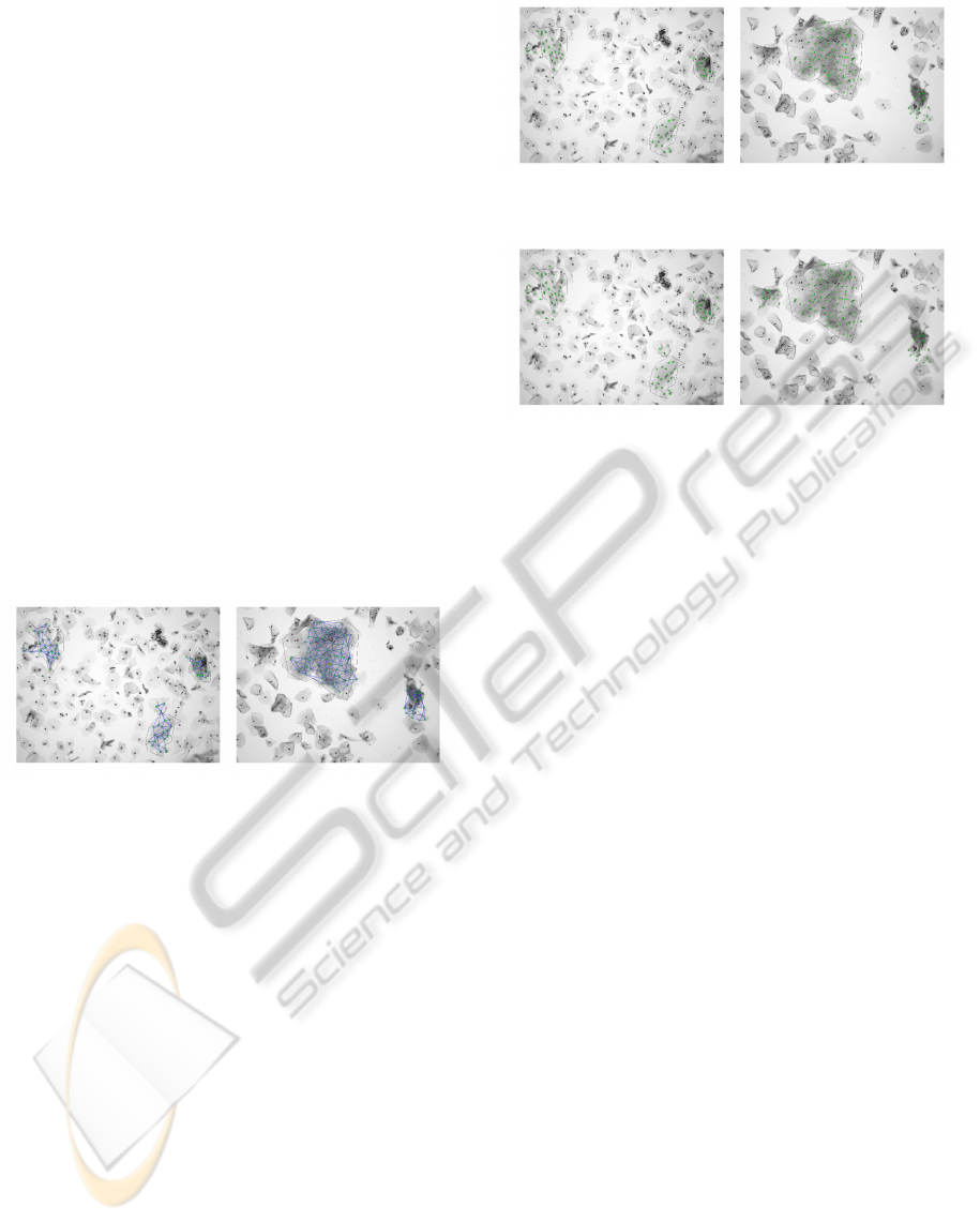
clustering with DT method. Figure 8 illustrates the

Figure 8: Detection of clusters using the intersection of

clustering methods results.

Figure 9: Detection of clusters using the union of clustering

methods results.

results obtained while detecting clusters using the in-

tersection of above-presented methods, and ﬁgure 9,

using the union.

Combined−U nion

= V

EMST

∪V

Delaunay

(6)

From both sets of vertices VCombined, we iden-

tify the different connected components (connected in

the Delaunay triangulation), in order to separate the

different clusters. We obtain several sets of vertices,

each set containing the vertices of a speciﬁc cluster.

4.4 Results

4.4.1 Ground Truth

The performance of the clustering methods was eval-

uated relative to manual deﬁnition of the clusters. A

Graphical User Interface (GUI) was developed to per-

mit a user to delineate regions containing clusters in

a set of images. A cervical cell image analysis expert

used the GUI to trace the clusters boundaries. A to-

tal of 48 images, belonging to different samples, have

been labelled and used to evaluate and compare the

methods. The accuracy of the methods is calculated

using the 48 images, containing a total of 2307 nu-

clei labelled as belonging to a cluster and 8116 nuclei

labelled as not belonging to a cluster.

4.4.2 The Cellgraph Method

In order to compare our method to the cellgraph based

method developed by Chandran et al. (Chandran

et al., 2012), we implemented that method using the

centroids of the segmented nuclei as a set V of ver-

tices of the graph. Some results using the cellgraph

ICPRAM2013-InternationalConferenceonPatternRecognitionApplicationsandMethods

362

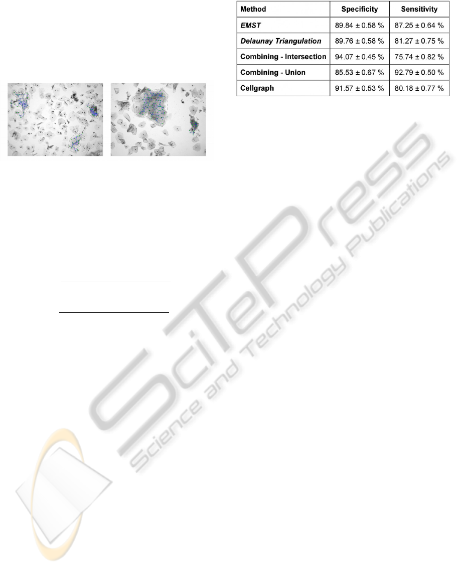
method are illustrated in ﬁgure 10. The cellgraph

method, as developed by Chandran et al., uses the

Waxman Model (Waxman, 1988), in which edges are

probabilistically assigned between vertices and the

probability of linking a pair of vertices v and w with

an edge decreases with the increase in the Euclidean

distance between them.

Figure 10: Detection of clusters using the cellgraph method.

4.4.3 Evaluation

Each method classiﬁes nuclei (or vertices) as belong-

ing to a cluster or not belonging to a cluster. To mea-

sure the performance of each method, we calculate

the sensitivity and speciﬁcity deﬁned as follow:

Speci f icity =

True Negative

True Negative + False Positive

× 100

(7)

Sensitivity =

True Positive

True Positive +False Negative

× 100

(8)

where a positive refers to a nucleus belonging to a

cluster and a negative, to a nucleus belonging to a

free-lying cell. True or false states the correctness of

the classiﬁcation in one of the two above mentioned

groups.

The speciﬁcity represents the probability that the

nucleus is classiﬁed as not in a cluster given that the

nucleus is indeed not in a cluster.

The sensitivity represents the probability that the

nucleus is classiﬁed as in a cluster given that the nu-

cleus is indeed in a cluster.

Figure 11 shows the resulting speciﬁcity and sen-

sibility for each method. As expected, speciﬁcity in-

creases and sensitivity decreases when using the in-

tersection of both methods and conversely, speciﬁcity

decreases and sensitivity increases when using the

union of both methods. Segmentation issues (nuclei

that had not been detected or that had been removed

after classiﬁcation, or artifacts that had been mistaken

as nuclei) often causes the methods to be imprecise

and improving the segmentation would beneﬁt to the

clustering results. It is also difﬁcult to deﬁne precisely

a cluster, and it was observed that some clusters de-

tected by the method, which had not been marked as

ground truth clusters, could actually be clusters.

Figure 11: Evaluation of the clustering methods with 95%

conﬁdence intervals.

5 CONCLUSIONS

In this paper, we presented a low resolution cell ﬁnd-

ing system for ﬁelds-of-view quality rating and clus-

ter detection in bright-ﬁeld microscope images of cer-

vical cells. Neighbourhood graphs have been ﬁt to

the image nuclei in order to model neighbourhood re-

lationships between cells. Transformations on such

graphs resulted in the detection of cell clusters and

the delineation of regions with varying degree of cell

density. The evaluation of our clustering methods in

term of sensitivity and speciﬁcity, as well as a com-

parison to a related work in the literature shows that

our approach is accurate, effective and relevant for the

detection of cells in clusters. We believe that the per-

formance of our methods can be further increased by

improving nuclei segmentation results.

REFERENCES

Bengtsson, E. (2005). Computerized cell image processing

in healthcare. In Choi, HK, editor, Healthcom 2005:

7th International Workshop on Enterprise Networking

and Computing in Healthcare Industry, Proceedings,

pages 11–17, 345 E 47TH ST, New York, NY 10017

USA. Korea Multimedia Soc; IEEE; Inje Univ; Busan

Convent Bur, IEEE. 7th International Workshop on

Enterprise Networking and Computing in Healthcare

Industry (HEALTHCOM 2005), Busan, South Korea,

JUN 23-25, 2005.

Chandran, S. P., Byju, N. B., Deepak, R. U., Kumar, R. R.,

Sudhamony, S., Malm, P., and Bengtsson, E. (2012).

Cluster detection in cytology images using the cell-

graph method. In IT in Medicine and Education

(ITME), 2012 International Symposium on.

Elsheikh, T. M., Austin, R. M., Chhieng, D. F., Miller, F. S.,

Moriarty, A. T., and Renshaw, A. A. (2012). American

society of cytopathology workload recommendations

for automated pap test screening: Developed by the

productivity and quality assurance in the era of auto-

mated screening task force. Diagnostic Cytopathol-

ogy, 1:1.

ClusterDetectionandField-of-ViewQualityRating-AppliedtoAutomatedPap-smearAnalysis

363

Grohs, H. and Husain, O., editors (1994). Automated Cervi-

cal Cancer Screening. IGAKU-SHOIN Medical Pub-

lishers, Inc.

Heijmans H., V. L. (1992). Mathematical Morphology in

Image Processing. CRC Press; First Edition edition,

New York.

Moshavegh, R., Ehteshami, B., Mehnert, A., Sujathan, K.,

Malm, P., and Bengtsson, E. (2012). Automated seg-

mentation of free-lying cell nuclei in pap smears for

malignancy-associated change analysis. In Engineer-

ing in Medicine and Biology Society (EMBC), 2012

Annual International Conference of the IEEE.

Nordin, B. (1989). The development of an automatic pre-

screener for the early detection of cervical cancer: Al-

gorithms and implementation. PhD thesis, Uppsala

University.

Papanicolaou, G. N., Traut, H. F., and Stanton A. Friedberg,

M. (1943). Diagnosis of uterine cancer by the vaginal

smear. Oxford University Press, New York.

Poulsen, R. S. (1973). Automated prescreening of cervical

cytology specimens. PhD thesis, Department of Elec-

trical Engineering, McGill University.

Raymond, E., Raphael, M., Grimaud, M., Vincent, L., Bi-

net, J. L., and Meyer, F. (1993). Germinal center anal-

ysis with the tools of mathematical morphology on

graphs. Cytometry, 14(8):848–61.

Saslow, D., Solomon, D., Lawson, H. W., Killackey, M.,

Kulasingam, S. L., Cain, J., Garcia, F. A. R., Moriarty,

A. T., Waxman, A. G., Wilbur, D. C., Wentzensen, N.,

Downs, L. S., Spitzer, M., Moscicki, A.-B., Franco,

E. L., Stoler, M. H., Schiffman, M., Castle, P. E., and

Myers, E. R. (2012). American cancer society, amer-

ican society for colposcopy and cervical pathology,

and american society for clinical pathology screening

guidelines for the prevention and early detection of

cervical cancer. American Journal of Clinical Pathol-

ogy, 137(4):516–542.

Vincent, L. (1989). Graphs and mathematical mor-

phology. Signal Processing, 16(4):365 – 388.

¡ce:title¿Special Issue on Advances in Mathematical

Morphology¡/ce:title¿.

Waxman, B. (1988). Routing of multipoint connections.

Selected Areas in Communications, IEEE Journal on,

6(9):1617 –1622.

WHO/ICO Information Centre on HPV and Cervical Can-

cer (HPV Information Centre) (2012). Human papillo-

mavirus and related cancers in world. summary report

2010.

Zuiderveld, K. (1994). Graphics gems iv. chapter Contrast

limited adaptive histogram equalization, pages 474–

485. Academic Press Professional, Inc., San Diego,

CA, USA.

ICPRAM2013-InternationalConferenceonPatternRecognitionApplicationsandMethods

364