Array-based Electromyographic Silent Speech Interface

Michael Wand, Christopher Schulte, Matthias Janke and Tanja Schultz

Cognitive Systems Lab, Karlsruhe Institute of Technology, Karlsruhe, Germany

Keywords:

EMG, EMG-based Speech Recognition, Silent Speech Interface, Electrode Array.

Abstract:

An electromygraphic (EMG) Silent Speech Interface is a system which recognizes speech by capturing the

electric potentials of the human articulatory muscles, thus enabling the user to communicate silently. This

study is concerned with introducing an EMG recording system based on multi-channel electrode arrays. We

ﬁrst present our new system and introduce a method to deal with undertraining effects which emerge due

to the high dimensionality of our EMG features. Second, we show that Independent Component Analysis

improves the classiﬁcation accuracy of the EMG array-based recognizer by up to 22.9% relative, which is

a ﬁrst example of an EMG signal processing method which is speciﬁcally enabled by our new array-based

system. We evaluate our system on recordings of audible speech; achieving an optimal average word error rate

of 10.9% with a training set of less than 10 minutes on a vocabulary of 108 words.

1 INTRODUCTION

Speech is the most convenient and natural way for

humans to communicate. Beyond face-to-face talk,

mobile phone technology and speech-based electronic

devices have made speech a wide-range, ubiquitous

means of communication. Unfortunately, voice-based

communication suffers from several challenges which

arise from the fact that the speech needs to be clearly

audible and cannot be masked, including lack of ro-

bustness in noisy environments, disturbance for by-

standers, privacy issues, and exclusion of speech-

disabled people.

These challenges may be alleviated by Silent

Speech Interfaces, which are systems enabling speech

communication to take place without the necessity of

emitting an audible acoustic signal, or when an acous-

tic signal is unavailable (Denby et al., 2010).

Over the past few years, we have developed a

Silent Speech Interface based on surface electromyo-

graphy (EMG): When a muscle ﬁber contracts, small

electrical currents in form of ion ﬂows are generated.

EMG electrodes attached to the subject’s face capture

the potential differences arising from these ion ﬂows.

This allows speech to be recognized even when it is

produced silently, i.e. mouthed without any vocal ef-

fort.

So far, all EMG-based speech recognizers have re-

lied on small sets of less than 10 EMG electrodes at-

tached to the speaker’s face (Schultz and Wand, 2010;

Maier-Hein et al., 2005; Freitas et al., 2012; Jor-

gensen and Dusan, 2010; Lopez-Larraz et al., 2010).

The technology is based on standard Ag-AgCl gelled

electrodes as used in medical applications. This setup

imposes some limitations, for example, small shifts in

the electrode positioning between recordings are difﬁ-

cult to compensate, and it is impossible to separate su-

perimposed signal sources, thus single active muscles

or motor units cannot be discriminated. In this paper,

we present ﬁrst results on using electrode arrays for

the recording of EMG signals of speech. We estab-

lish a baseline procedure to allow an existing state-

of-the-art EMG-based continuous speech recognizer

(Schultz and Wand, 2010) to deal with the increased

number of signal channels, and we present a ﬁrst

application of the EMG array methodology, namely,

we show that application of Independent Component

Analysis (ICA) reduces the Word Error Rates of the

recognizer.

In the future, we expect EMG array technology to

allow a much more ﬁne-grained EMG-based recogni-

tion of articulatory activity than can be achieved with

separate-electrode systems: The multi-channel sig-

nal will allow us to perform source separation meth-

ods, as presented in this paper, and should offer the

possibility to extract and model certain articulatory

patterns which are part of the human speech pro-

cess. In terms of practical usage, the setup time for

the new system is signiﬁcantly shorter than for the

old separate-electrode system, since the electrode at-

Wand M., Schulte C., Janke M. and Schultz T..

Array-based Electromyographic Silent Speech Interface.

DOI: 10.5220/0004252400890096

In Proceedings of the International Conference on Bio-inspired Systems and Signal Processing (BIOSIGNALS-2013), pages 89-96

ISBN: 978-989-8565-36-5

 2013 SCITEPRESS (Science and Technology Publications, Lda.)

Figure 1: EMG array positioning for setup A (left) and setup

B (right).

tachment process is much shorter than for separate-

electrode systems.

The remainder of this paper is organized as fol-

lows: In the following section 2, we describe our new

recording system, and section 3 contains a description

of the underlying decoding system. Section 4 presents

our experiments, and the ﬁnal section 5 concludes the

paper.

2 RECORDING SYSTEM SETUP

AND CORPUS

For EMG recording we used the multi-channel

EMG ampliﬁer EMG-USB2 produced and dis-

tributed by OT Bioelettronica, Italy (http://www.

otbioelettronica.it/). The EMG-USB2 ampli-

ﬁer allows to record and process up to 256 EMG chan-

nels, supporting a selectable gain of 100 - 10000 V/V

and a recording bandwidth of 3 Hz - 4400 Hz. For line

interference reduction, we used the integrated DRL

circuit (Winter and Webster, 1983). The electrode ar-

rays were acquired from OT Bioelettronica as well.

Electrolyte cream was applied to the EMG arrays in

order to reduce the electrode/skin impedance.

We used two different EMG array conﬁgurations

for our experiments, see ﬁgure 1. In setup A, we

unipolarly recorded 16 EMG channels with two EMG

arrays each featuring a single row of 8 electrodes,

with 5 mm inter-electrode distance (IED). One of the

arrays was attached to the subject’s cheek, captur-

ing several major articulatory muscles (Maier-Hein

et al., 2005), the other one was attached to the sub-

ject’s chin, in particular recording signals from the

tongue. A reference electrode was placed on the sub-

ject’s neck.

In setup B, we replaced the cheek array with a

larger array containing four rows of 8 electrodes, with

10 mm IED. The chin array remained in its place. In

this setup, we achieved a cleaner signal by using a

bipolar conﬁguration, where the potential difference

between two adjacent channels in a row is measured.

This means that out of 4 × 8 cheek electrodes and 8

chin electrodes, we obtain (4+1)·7 = 35 signal chan-

nels.

For both setups, we chose an ampliﬁcation factor

of 1000, a high-pass ﬁlter with a cutoff frequency of

3 Hz and a low-pass ﬁlter with a cutoff frequency of

900 Hz, and a sampling frequency of 2048 Hz. The

audio signal was parallely recorded with a standard

close-talking microphone. We used an analog marker

system to synchronize the EMG and audio recordings,

and according to (Jou et al., 2006), we delayed the

EMG signal by 50ms compared to the audio signal.

The text corpus which we recorded is based on

(Schultz and Wand, 2010). We used two different text

corpora for our recordings: Each session contains a

set of ten “BASE” sentences which is used for test-

ing and kept ﬁxed across sessions. Furthermore, each

session contains 40 test sentences, which vary across

sessions. For reference, we call this basic text corpus

“Set 1”. A subset of our sessions has been extended to

160 different training sentences and 20 test sentences,

where the 20 test sentences consist of the BASE set

repeated twice. This enlarged text corpus is called

“Set 2”.

The recording proceeded as follows: In a quiet

room, the speaker read English sentences in normal,

audible speech. The recording was supervised by a

member of the research team in order to detect errors

(e.g. detached electrodes) and to assure a consistent

pronunciation. The training and test sentences were

always recorded in randomized order. Thus we ﬁnally

have four setups to investigate, namely, setups A-1

and A-2 (with 16 EMG channels) and B-1 and B-2

(with 35 EMG channels). At this point we remark that

the results on the four setups are not directly compara-

ble, since the number of training sentences, the set of

speakers and the number of sessions per speaker dif-

fer. Also, our experience indicates that even for one

single speaker, the recognition performance may vary

drastically between sessions, possibly due to varia-

tions in electrode positioning, skin properties, etc.

However, it is certainly plausible to compare the ef-

fects of different feature extraction methods on the

recognition performance of each of the setups, which

is the purpose of this paper. It should also be noted

that the test sets of the four setups exhibit identical

characteristics in terms of perplexity and vocabulary.

The following table summarizes the properties of

our corpus.

Setup # of Speakers / Average data length in sec.

Sessions Training Test Total

A-1 3 / 6 144 37 181

A-2 2 / 2 528 74 602

B-1 6 / 7 149 42 191

B-2 4 / 4 570 83 653

BIOSIGNALS2013-InternationalConferenceonBio-inspiredSystemsandSignalProcessing

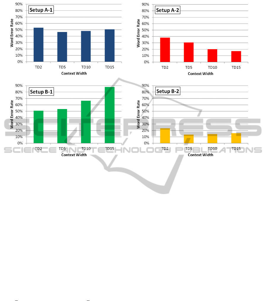
Figure 2: Word Error Rates for the baseline system with different stacking context widths (no PCA or ICA).

3 FEATURE EXTRACTION,

TRAINING AND DECODING

The feature extraction is based on time-domain fea-

tures (Jou et al., 2006). We ﬁrst split the incom-

ing EMG signal channels into a high-frequency and

a low-frequency part, after this, we perform framing

and compute the features, as follows:

For any given feature f,

f is its frame-based time-

domain mean, P

is its frame-based power, and z

is its

frame-based zero-crossing rate. S(f, n) is the stacking

of adjacent frames of feature f in the size of 2n + 1

(−n to n) frames.

For an EMG signal with normalized mean x[n], the

nine-point double-averaged signal w[n] is deﬁned as

w[n] =

∑

k=−4

v[n + k], where v[n] =

∑

k=−4

x[n + k].

The high-frequency signal is p[n] = x[n] − w[n],

and the rectiﬁed high-frequency signal is r[n] = |p[n]|.

The ﬁnal feature TDn is deﬁned as follows:

TDn = S(TD0, n), where TD0 = [

w, P

, P

, z

r],

i.e. a stacking of adjacent feature vectors with con-

text width 2 · n + 1 is performed, with varying n. This

process is performed for each channel, and the com-

bination of all channel-wise feature vectors yields the

ﬁnal TDn feature vector. Frame size and frame shift

are set to 27 ms respective 10 ms.

In all cases, we apply Linear Discriminant Anal-

ysis (LDA) on the TDn feature. The LDA ma-

trix is computed by dividing the training data into

136 classes corresponding to the begin, middle, and

end parts of 45 English phonemes, plus one si-

lence phoneme. From the 135 dimensions which

are yielded by the LDA algorithm, we always re-

tain 32 dimensions, which is in line with previous

work (Jou et al., 2006; Schultz and Wand, 2010) and

thus allows to compare our performance with the re-

sults on single-electrode systems. Preliminary exper-

iments with a higher number of retained dimensions

did not show any signiﬁcant improvement. As shown

in section 4.2, it may be necessary to perform Prin-

cipal Component Analysis (PCA) before computing

the LDA matrix, see section 4.2 for further details. In

the experiments described in section 4.3, Independent

Component Analysis (ICA) is applied before the fea-

ture extraction step, on the raw EMG data.

The recognizer is based on three-state left-to-right

fully continuous Hidden-Markov-Models. All exper-

iments used bundled phonetic features (BDPFs) for

training and decoding, see (Schultz and Wand, 2010)

for a detailed description. In order to obtain phonetic

time-alignments as a reference for training, the paral-

lely recorded acoustic signal was forced-aligned with

Array-basedElectromyographicSilentSpeechInterface

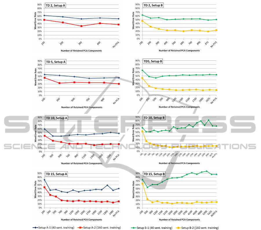
Figure 3: Word Error Rates for different PCA dimension reductions. Observe that the feature space dimension before the

PCA step increases from left to right and from top to bottom.

an English Broadcast News (BN) speech recognizer.

Based on these time-alignments, the HMM states are

initialized by a merge-and-split training step (Ueda

et al., 2000), followed by four iterations of Viterbi

training.

For decoding, we used the trained acoustic model

together with a trigram Broadcast News language

model. The test set perplexity is 24.24. The decod-

ing vocabulary was restricted to the words appearing

in the test set, which resulted in a test vocabulary of

108 words. Note that we do not use lattice rescoring

for our experiments.

4 EXPERIMENTS AND RESULTS

In this section we ﬁrst outline our baseline system,

based on (Schultz and Wand, 2010), and then de-

scribe the modiﬁcations to the feature extraction pro-

cess which are necessary to deal with a large number

of channels. In the ﬁnal part, we apply Independent

Component Analysis (ICA) to the raw EMG data and

show that it can increase the recognition accuracy.

4.1 Baseline Recognition System

Our ﬁrst experiment establishes a baseline recogni-

tion system. We use our recognizer, as described in

section 3, and feed it with the EMG features from the

BIOSIGNALS2013-InternationalConferenceonBio-inspiredSystemsandSignalProcessing

Table 1: Optimal Results and Parameters with and without PCA.

Setup A-1 A-2 B-1 B-2

Best Result without PCA (“Baseline”) 46.3% 17.0% 50.5% 13.4%

Optimal Stacking Width without PCA 5 15 2 5

Optimal Number of Dimensions without PCA 880 2480 875 1925

Best Result with PCA 40.1% 13.9% 44.9% 10.9%

Optimal Stacking Width with PCA 15 15 5 10

Optimal Number of Dimensions with PCA 900 2480 500 1500

Relative Improvement by PCA Application 13.4% 18.2% 11.1% 18.7%

array recording system. Figure 2 shows the Word Er-

ror Rates for different stacking widths, averaged over

all sessions of the four setups.

We now consider the optimal context widths for

the four setups. This has been investigated e.g. by

(Jou et al., 2006), where a context width of 5 was

used, and by (Wand and Schultz, 2010), where it was

shown that increasing the context width to 15 frames,

i.e. 150 ms, still brings some improvement.

Our observations for the four distinct setups pre-

sented in this study are very different: For setup A-

1, with 16 channels and 40 training sentences, the

Word Error Rate (WER) varies between 46.3% and

53.2%, with the optimum reached at a context width

of 5 (i.e. TD5). For the B-1 setup, with 35 channels

but the same amount of training data, the optimal con-

text width appears to be TD2 with a WER of 50.5%,

and for wider contexts, which increases to 87.6% for

the TD15 stacking.

For the setups with 160 training sentences, the

recognition performance is generally better due to the

increased training data amount. With respect to con-

text widths, we observe a behavior which vastly dif-

fers from the results above: For 16 EMG channels

(setup A-2), the optimal context width is TD15, with

a WER of only 17.0%. For setup B-2, TD5 stacking

is optimal, with a WER of 13.4%.

The behavior described in this section is quite con-

sistent across recording sessions. This means that

even though the corpora for the four setups are dif-

ferent, we have observed a deep inconsistency with

respect to the optimal stacking width, which leads us

to the series of experiments described in the following

section.

4.2 PCA Preprocessing to avoid LDA

Sparsity

Machine learning tasks frequently exhibit a chal-

lenge known as the “Curse of Dimensionality”, which

means that high-dimensional input data, relative to

the amount of training data, causes undertraining, di-

minishes the effectiveness of machine learning algo-

rithms, and reduces in particular the generalization

capability of the generated models. The maximal fea-

ture space dimension which allows robust training de-

pends on the amount of available training data.

The dimensionality of the feature space in our

experiments depends on the number of EMG chan-

nels and the stacking width during feature extraction.

From the results of section 4.1, we observe

• that for both setups A and B, increasing the

amount of training data increases the optimal con-

text width

• and that for both the 40-sentence training corpus

(set 1) and the 160-sentence training corpus (set

2), the optimal context width with setup B is lower

than the optimum for setup A.

This strongly suggests that the “Curse of Dimension-

ality” is the cause of the discrepancy we observed.

However, since the LDA algorithm always reduces

the feature space dimensionality to 32 channels, the

GMM training itself is not affected by varying feature

dimensionalities.

We assumed that the deterioration of recognition

accuracy for small amounts of training data and high

feature space dimensionalities is caused by the LDA

computation step. It has been shown that when the

amount of training data is small relative to the sam-

ple dimensionality, the LDA within-scatter matrix be-

comes sparse, which reduces the effectivity of the

LDA algorithm (Qiao et al., 2009). This may be the

case in our setup, since with only a few minutes of

training data, we may have a sample dimensionality

before LDA of up to 35 · 5 · 31 = 5425 for the 35-

channel system with a TD15 stacking.

The following set of experiments deals with cop-

ing with the LDA sparsity problem. From these ex-

periments we expect an improved recognition accu-

racy and, in particular, a more consistent result re-

garding the optimal feature stacking width. In these

experiments, we allowed an additional PCA dimen-

sion reduction step before the LDA computation,

as advocated for visual face recognition (Belhumeur

et al., 1997). This step should allow an improved

LDA estimation, however, if the PCA cutoff dimen-

sion is chosen too low, one will lose information

Array-basedElectromyographicSilentSpeechInterface

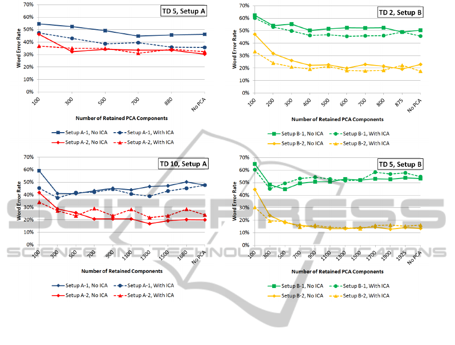
Figure 4: Word Error Rates after ICA application, for the four different setups and varying context widths.

which is important for discrimination.

The computation works as follows: On the train-

ing data set, we ﬁrst compute a PCA transformation

matrix. We apply PCA and keep a certain number

of components from the resulting transformed sig-

nal, where the components are, as usual, sorted by

decreasing variance. Then we compute an LDA ma-

trix of the PCA-transformed training data set, ﬁnally

keeping 32 dimensions. The resulting PCA + LDA

preprocessing is now applied to the entire corpus, nor-

mal HMM training and testing is performed, and we

use the Word Error Rate as a measure for the quality

of our preprocessing.

Figure 3 plots the Word Error Rates of our recog-

nizer for setups A and B and different stacking widths

versus the number of retained dimensions after the

PCA step. In all cases, we jointly plot the WERs for

training data sets 1 and 2.

The ﬁgures show that the PCA step indeed helps

to overcome LDA sparsity. For example, in the A-1

setup, the optimal context width without PCA appli-

cation is 5, yielding a WER of 46.3%. With PCA

application, the optimal number of retained PCA di-

mensions for the TD5 context width is 700, yielding a

WER of 44.8%. However, we can still do better: With

a vastly increased context width of 15, we get the best

WER of 40.1%, at a dimensionality after PCA appli-

cation of 900.

This is also true for the other four setups, see ta-

ble 1 for an overview. In all cases, we obtain WER

reductions of more than 10% relative, and also, in all

cases the optimal context width increases.

So far, we have found the optimal context width

for the EMG speech classiﬁcation task to lie around

10 to 15 frames on each side, which makes a context

of around 200-300 ms. It may be possible to try even

wider contexts, however, close examination of the re-

sults in ﬁgure 3 show that between the context widths

of 10 and 15, the respective results with optimal PCA

dimensionality are rather close for each of the four

setups.

4.3 ICA Application

Having established a baseline recognizer, we now turn

our attention to applications of array technology. One

well-established means of identifying signal sources

in multi-channel signals is Independent Component

Analysis (ICA) (Hyvrinen and Oja, 2000). ICA is a

linear transformation which is used to obtain indepen-

dent components within a multi-channel signal; the

underlying idea is that the statistical independence be-

BIOSIGNALS2013-InternationalConferenceonBio-inspiredSystemsandSignalProcessing

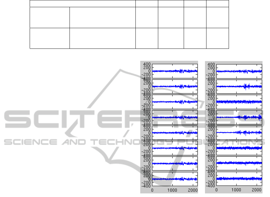
Table 2: Best Results with and without ICA.

Setup A-1 A-2 B-1 B-2

Without PCA

Best Result without ICA 46.3% 17.0% 50.5% 13.4%

Best Result with ICA 35.7% 16.2% 44.2% 12.1%

Relative Improvement 22.9% 4.7% 12.5% 9.7%

With PCA

Best Result without ICA 40.1% 15.15% 44.9% 10.9%

Best Result with ICA 35.7% 12.40% 40.8% 11.8%

Relative Improvement 11.0% 18.2% 9.1% -8.3%

tween the estimated components is maximized.

We interpret ICA as a method of (blind) source

separation, therefore we apply ICA and then run our

recognizer on the estimated components; this includes

the PCA step and the LDA step. Another method

would be to delete undesired sources, e.g. noise, and

then back-project the remaining components (Jung

et al., 2000). Also, we do not manually remove un-

desired channels, instead we allow the PCA+LDA

step to remove these non-discriminative components.

Clearly, this is expected to be only a ﬁrst step towards

a more meticulous application of ICA, in particular,

we expect to be able to detect and remove irrelevant

noise channels in the future.

The ICA separation matrix is always computed on

the training data of the respective sessions. Since in

both setups A and B, we have two separate EMG

arrays, we run the ICA algorithm on the channels

from these two arrays separately. We use the Info-

max ICA algorithm according to (Bell and Sejnowski,

1995), as implemented in the Matlab EEGLAB tool-

box (Makeig, S. et al., 2000).

Figure 4 shows average Word Error Rates for se-

tups A and B, plotted against the PCA cutoff dimen-

sion, with and without ICA application. As typical

examples of our observations, for setup A we plotted

the results for the context widths of 5 and 10, for setup

B, we chose the context widths of 2 and 5.

It can be seen that in almost all cases, ICA im-

proves the recognition results consistently across dif-

ferent PCA dimensionalities. The remarkable excep-

tions are setups B-1 and B-2 with TD5 stacking. Gen-

erally, ICA appears to be slightly more helpful in

setup A. Table 2 gives an overview of the results of

ICA application. It can be seen that the only case

where ICA application gives a worse result is the B-

2 setup, which is, however, still our best setup alto-

gether.

Finally, we ask the question why the ICA appli-

cation does not yet always yield satisfactory results.

One can visually study the effects of ICA preprocess-

ing by looking at the EMG signals before and after

ICA application: Figure 5 gives a typical example of

the ﬁrst second of a recording from corpus A-2; only

the signals from the cheek array are shown. One sees

Figure 5: 8-channel EMG signals before ICA application

(left) and after ICA application (right).

that the eight original channels (left) show somewhat

similar patterns, including a relatively large amount

of pure noise at the beginning, when the speaker has

not yet started to articulate.

The ICA-processed signals present a different im-

age: Out of the eight channels, four show white noise

throughout the recording, three show starkly different

EMG signals, and the ﬁrst channel appears to show

a mixture of noise and content-bearing signal. Note

that the ICA implementation changes the scale of the

ICA components.

Our current method applies the EMG preprocess-

ing described in section 3 to all these ICA components

indiscriminately. The fact that the recognition results

are better for the ICA-processed signals than for the

original EMG data indicates that the PCA+LDA step

is able to suppress the noise components and concen-

trates on the content-bearing channels, however, this

method is likely suboptimal. In the future we plan to

develop and apply heuristical methods to distinguish

content-bearing signals and noise components, so that

the latter can be automatically removed.

Array-basedElectromyographicSilentSpeechInterface

5 CONCLUSIONS

In this study we have laid the basics of a new EMG-

based speech recognition technology, based on elec-

trode arrays instead of single electrodes. We have

presented two basic recognition setups and evaluated

their potential on data sets of different sizes. The

unexpected inconsistency with respect to the optimal

stacking width led us to the introduction of a PCA

preprocessing step before the LDA matrix is com-

puted, which gives us consistent relative Word Error

Rate improvements of 10% to 18%, even for small

training data sets of only 40 sentences.

As a ﬁrst application of the new array technology,

we have shown that Independent Component Analy-

sis (ICA) typically improves our recognition results.

We also have observed that our method of applying

ICA does not yet always yield satisfactory results: In

one of our setups, we actually observed slightly worse

results than without ICA.

REFERENCES

Belhumeur, P. N., Hespanha, J. P., and Kriegman, D. J.

(1997). Eigenfaces vs Fisherface: Recognition using

Class-speciﬁc Linear Projection. IEEE Transactions

on Pattern Analysis and Machine Intelligence, 19:711

– 720.

Bell, A. J. and Sejnowski, T. I. (1995). An Information-

Maximization Approach to Blind Separation and

Blind Deconvolution. Neural Computation, 7:1129 –

1159.

Denby, B., Schultz, T., Honda, K., Hueber, T., and Gilbert,

J. (2010). Silent Speech Interfaces. Speech Commu-

nication, 52(4):270 – 287.

Freitas, J., Teixeira, A., and Dias, M. S. (2012). Towards

a Silent Speech Interface for Portuguese. In Proc.

Biosignals.

Hyvrinen, A. and Oja, E. (2000). Independent Component

Analysis: Algorithms and Applications. Neural Net-

works, 13:411 – 430.

Jorgensen, C. and Dusan, S. (2010). Speech Interfaces

based upon Surface Electromyography. Speech Com-

munication, 52:354 – 366.

Jou, S.-C., Schultz, T., Walliczek, M., Kraft, F., and Waibel,

A. (2006). Towards Continuous Speech Recogni-

tion using Surface Electromyography. In Proc. Inter-

speech, pages 573 – 576, Pittsburgh, PA.

Jung, T., Makeig, S., Humphries, C., Lee, T., Mckeown, M.,

Iragui, V., and Sejnowski, T. (2000). Removing Elec-

troencephalographic Artifacts by Blind Source Sepa-

ration. Psychophysiology, 37:163 – 178.

Lopez-Larraz, E., Mozos, O. M., Antelis, J. M., and

Minguez, J. (2010). Syllable-Based Speech Recog-

nition Using EMG. In Proc. IEEE EMBS.

Maier-Hein, L., Metze, F., Schultz, T., and Waibel, A.

(2005). Session Independent Non-Audible Speech

Recognition Using Surface Electromyography. In

IEEE Workshop on Automatic Speech Recognition

and Understanding, pages 331 – 336, San Juan,

Puerto Rico.

Makeig, S. et al. (2000). EEGLAB: ICA Toolbox for Psy-

chophysiological Research. WWW Site, Swartz Cen-

ter for Computational Neuroscience, Institute of Neu-

ral Computation, University of San Diego California:

www.sccn.ucsd.edu/eeglab/.

Qiao, Z., Zhou, L., and Huang, J. Z. (2009). Sparse Lin-

ear Discriminant Analysis with Applications to High

Dimensional Low Sample Size Data. International

Journal of Applied Mathematics, 39:48 – 60.

Schultz, T. and Wand, M. (2010). Modeling Coarticulation

in Large Vocabulary EMG-based Speech Recognition.

Speech Communication, 52(4):341 – 353.

Ueda, N., Nakano, R., Ghahramani, Z., and Hinton, G. E.

(2000). Split and Merge EM Algorithm for Improving

Gaussian Mixture Density Estimates. Journal of VLSI

Signal Processing, 26:133 – 140.

Wand, M. and Schultz, T. (2010). Speaker-Adaptive Speech

Recognition Based on Surface Electromyography. In

Fred, A., Filipe, J., and Gamboa, H., editors, Biomedi-

cal Engineering Systems and Technologies, volume 52

of Communications in Computer and Information Sci-

ence, pages 271–285. Springer Berlin Heidelberg.

Winter, B. B. and Webster, J. G. (1983). Driven-right-leg

Circuit Design. IEEE Trans. Biomed. Eng., BME-

30:62 – 66.

BIOSIGNALS2013-InternationalConferenceonBio-inspiredSystemsandSignalProcessing