A Methodology for Optimizing the Cost Matrix in Cost Sensitive

Learning Models applied to Prediction of Molecular Functions

in Embryophyta Plants

S. Garc

ıa-L

opez

, J. A. Jaramillo-Garz

1,2

, L. Duque-Mu

noz

1,2

and C. G. Castellanos-Dom

ınguez

Signal Processing and Recognition Group, Universidad Nacional de Colombia,

Campus la Nubia, Km 7 v

ıa al Magdalena, Manizales, Colombia

Grupo de M

aquinas Inteligentes y Reconocimiento de Patrones - MIRP, Instituto Tecnol

ogico Metropolitano,

Cll 54A No 30-01, Medell

ın, Colombia

Keywords:

Molecular Functions Prediction, Proteins, Cuckoo Search, Cost Sensitive Learning, Class Imbalance.

Abstract:

Due to the large amount of data generated by genomics and proteomics research, the use of computational

methods has been a great support tool for this purpose. However, tools based on machine learning, face

several problems associated to the nature of the data, one of them is the class-imabalance problem. Several

balancing techniques exist to obtain an improvement in prediction performance, such as boosting and resam-

pling, but they have multiple weaknesses in difﬁcult data spaces. On the other hand, cost sensitive learning

is an alternative solution, yet, the obtention of appropriate cost matrix to induce a good prediction model is

complex, and still remains an open problem. In this paper, a methodology to obtain an optimal cost matrix to

train models based on cost sensitive learning is proposed. The results show that cost sensitive learning with a

proper cost can be very competitive, and even outperform many class-balance strategies in the state of the art.

Tests were applied to prediction of molecular functions in Embryophyta plants.

1 INTRODUCTION

Modern biology has seen an increasing use of com-

putational techniques for large scale and complex

biological data analysis. Various computational

techniques, particularly machine learning algorithms

(Larra

naga et al., 2006) are applied to identify func-

tions of gene products speciﬁed by the molecular ac-

tivities they perform. In this context, there is a vast

number of problems associated with the nature of the

data. In particular, given that the same protein can

be associated to several functional classes, a problem

of classiﬁcation with multiple labels is generated. A

straightforwad way to solve this kind of problem is the

“one-against-all” strategy, in wich a binary classiﬁer

is trained per each class, in order to take independent

decisions about the membership of proteins. Yet, this

approach leads to a high degree of imbalance between

the number of samples in each class, magnifying the

already present disparity in their sizes and thereby

producing a large bias towards the category with more

information (Sonnenburg et al., 2007). There are sev-

eral ways to address class imbalance problems. Tech-

niques like Sampling and Boosting offer different so-

lutions to same issue, either from the addiction of

subtraction of samples to balance class distribution

(He and Garcia, 2009), or by the training of individ-

ually trained classiﬁers in an iterative way in order

to emphasizes on the incorrectly learned instances by

the previous iteration trained classiﬁer (Ding, 2011).

However, these techniques have some drawbacks, be-

tween them, the over-training and noise addition in

the training set (oversampling), the lost of useful

data if a reliable sample selection criteria is not se-

lected (subsampling), tendency to fail if there not ex-

ist enough data or the inability to be a good model

in the presence of noise in the training set (Boost-

ing) (He and Garcia, 2009). By the other hand, mod-

els based on cost sensitive learning assume different

costs (or penalties) when examples are misclassiﬁed

from one category to another. This process is mod-

elled by a cost matrix that is a numerical representa-

tion of the penalty of classifying examples from one

category to another. Conventionally, models based on

cost-sensitive learning assume that the costs are ﬁxed,

but this condition is not met in real-world applications

and this is still an open problem (Liu and Zhou, 2012).

In this paper, a simple and efﬁcient methodology

García-López S., A. Jaramillo-Garzón J., Duque-Muñoz L. and G. Castellanos-Domínguez C..

A Methodology for Optimizing the Cost Matrix in Cost Sensitive Learning Models applied to Prediction of Molecular Functions in Embryophyta Plants.

DOI: 10.5220/0004250900710080

In Proceedings of the International Conference on Bioinformatics Models, Methods and Algorithms (BIOINFORMATICS-2013), pages 71-80

ISBN: 978-989-8565-35-8

 2013 SCITEPRESS (Science and Technology Publications, Lda.)

for obtaining the optimal cost matrix of a cost sensi-

tive learning model is proposed. This methodology

is applied to the prediction of molecular functions in

Embryophyta plants and is compared with a broad

spectrum of class-balance strategies in order to obtain

a comprehensive analysis of the problem. The results

show that cost sensitive models are highly reliable and

can outperform many commonly used balance strate-

gies in the prediction of molecular functions.

2 CLASS-BALANCE

STRATEGIES

This section describes the principles of all the com-

monly used class-balance strategies that are going to

be used in the experiments below. They are divided

into three categories: sampling strategies, boosting

strategies and cost sensitive strategies.

2.1 Sampling Strategies

2.1.1 Synthetic Minority Oversampling Method

(SMOTE)

SMOTE is an oversampling method proposed in

(Chawla et al., 2002), which main idea is to create

new synthetic samples that will belong to the minor-

ity class. These samples are computed by interpola-

tion among several closely spaced real samples. In

this way, the decision boundary of the minority class

becomes more general (Grzymala-Busse et al., 2005).

The synthetic samples are generated as follows: for

each real sample under consideration, represented as

a feature vector, the distance between it and its near-

est neighbors is taken. The result is multiplied by a

random number between 0 to 1 with a uniform prob-

ability, and this result is added to the original feature

vector. This procedure causes the selection of a ran-

dom point along the line segment between two sam-

ples. The SMOTE algorithm can be seen in (Chawla

et al., 2002).

2.1.2 Subsampling based on Particle Swarm

Optimization

This technique is based on the search of an opti-

mal sample subset for majority class, that maximizes

the generalization capability of the classiﬁer. To this

purpose, a metaheuristic optimization strategy known

as Particle Swarm Optimization (PSO) is used. The

main concept of this technique is synthesized in the

following form: To a given dataset, a cross valida-

tion composed by three folds is used, generating ex-

ternal training and test sets. This external training sets

are partitioned in turn with another cross-validation of

three folds, these being the internal validation sets.

In this internal validation set, the internal training

sets are used to resampling, while internal test sets

guide the optimization process. Then the external test

sets are reserved to the balance set evaluation and ex-

cluded from resample process. The hybrid optimiza-

tion system based on PSO is used to evaluate the merit

of each majority class sample to compensate the bal-

ance effect between them. This is achieved through

the creation of different samples subsets of majority

class combined with the minority class to build a clas-

siﬁcation model which is them used to the partition of

test classiﬁcation. When the completion criterion is

accomplished, the selected samples by the last itera-

tion are ordered by their frequency selection. After

the list of frequencies of selected samples is obtained,

a balanced dataset from the combination of the sam-

ples belonging to majority class with major frequency

index and samples of minority class is constructed

(Yang et al., 2009). the process of this algorithm is

explained in greater detail in (Yang et al., 2009).

2.2 Boosting Strategies

2.2.1 AdaBoost

Boosting algorithms are iterative algorithms that

place different weights on the training distribution at

each iteration. After each iteration, boosting increases

the weights associated with incorrectly classiﬁed ex-

amples and decreases the weights associated with cor-

rectly classiﬁed examples. This forces the system to

focus on the rare items, incrementing the weights as-

signed to rare classes. The most representative tech-

nique belonging to Boosting algorithms is AdaBoost

(Polikar, 2006). AdaBoost generates a set of clas-

siﬁers, and combines them through weighted major-

ity voting of the classes predicted by the individual

hypotheses. The hypotheses are generated by train-

ing a weak classiﬁer, using instances drawn from an

iteratively updated distribution of the training data.

This distribution update ensures that instances mis-

classiﬁed by the previous classiﬁer are more likely to

be included in the training data of the next classiﬁer.

Hence, consecutive classiﬁers training data are geared

towards increasingly hard-to-classify instances (Po-

likar, 2006), (Schapire, 1999). AdaBoost takes the

ﬁnal decision via weighted majority voting, i.e, each

classiﬁer will have a different power of decision, it de-

pends on the performance during training procedure,

as the classiﬁer has better performance, will be fa-

vored with a greater power of decision over the other

BIOINFORMATICS2013-InternationalConferenceonBioinformaticsModels,MethodsandAlgorithms

classiﬁers (Polikar, 2006). The algorithm is explained

in a detailed way in (Schapire, 1999).

2.3 Cost Sensitive Strategies

2.3.1 Cost Sensitive Learning

This strategy attempts to minimize costs (or maxi-

mize proﬁts) associated with its decisions rather than

simply getting a high precision. In biclass problems,

when misclassiﬁed samples of one class are much

more costly than misclassiﬁed samples of another

class, it generate a model that center more in the cor-

rect classiﬁcation of sample of the most costly class

samples than a model where the class treated equally.

Given a costs speciﬁcation for correct and incorrect

predictions, a sample could be predicted to have the

class that leads to lower expected cost, where the ex-

pected value is computed using conditional probabil-

ity of each class given a sample. Mathematically be

(i, j) the inputs associated to a cost matrix C, where C

have the cost to predict a class i when the true class is

j. If i = j, then the prediction is correct, while if i 6= j,

the prediction is incorrect. The optimal prediction for

a sample is the class that minimize:

L(x,i) =

∑

P( j|x)C(i, j)

Where cost matrix C(i, j) is deﬁned as:

Table 1: Cost matrix.

Actual negative Actual positive

Predict negative C(0,0) = c

C(0, 1) = c

Predict positive C(1,0) = c

C(1, 1) = c

For each i, L(x,i) is the sum over the alternative

possibilities for the true class of x. In this framework,

the goal of algorithm based on cost sensitive learning

is to produce a classiﬁer that can estimate the proba-

bility P( j|x) given any example x, being this the true

class of x. For an example x, i means make the pre-

diction act as if i was the true class of x. the essence

decision-making by cost sensitivity is that this may

be optimal to act as if a class is true even when other

classes are more likely (Elkan, 2001). In biclass case,

the optimal prediction will be the class 1 if and only

if the expected cost of the prediction is less than or

equal to the expected cost of predicting class 0, i.e:

P( j = 0|x)c

+ P(j = 1|x)c

< P( j = 0|x)c

+ P( j = 1|x)c

Which equals to:

(1 − p)c

+ pc

< (1 − p)c

+ pc

where p = P( j = 1|x)

The threshold for optimal decision making is such

that:

∗

− c

+ c

− c

2.3.2 MetaCost

The basic idea of MetaCost is to take a normal, unal-

tered classiﬁer and adjust the learning with a cost ma-

trix. First, the training set is taken to form multiples

subsets via bootstrap. each subset create by bootstrap

is used to build a ensemble of classiﬁers to take the

ﬁnal decision, where each subsets and classiﬁers are

equals to number of iteration used in MetaCost. The

ensemble of classiﬁers are then combined through a

majority vote to determine the probability of each data

object x belonging to each class label. Next, each data

object in the training data is relabeled based on the

evaluation of a conditional risk function, and a ﬁnal

classiﬁer is then produced after applying the classiﬁ-

cation algorithm to the relabeled training data. The

conditional risk function is deﬁned as:

R(i|x) =

∑

P( j|x)C

i, j

(1)

Where the conditional risk determine the cost of

predicting that sample x belongs to class label i in-

stead of class label j, P( j|x) is the conditional prob-

ability that sample x belongs to label j, and C

i, j

the cost matrix used in the classiﬁcation (Domin-

gos, 1999). The Algorithm is explained in detail in

(Domingos, 1999)

3 PROPOSED METHOD:

OPTIMAL COST MATRIX

SEARCH VIA CUCKOOCOST

This section describes the theoretical background and

foundations of the proposed methodology for select-

ing the optimal cost matrix.

3.1 Cuckoo Search

Cuckoo Search is based on the parasitic behavior ex-

posed by some species of Cuckoo birds. His natu-

ral strategy consist in leave eggs in host nest created

by other birds. This eggs presents the particularity to

AMethodologyforOptimizingtheCostMatrixinCostSensitiveLearningModelsappliedtoPredictionofMolecular

FunctionsinEmbryophytaPlants

have a big similitude with host eggs, the more similar

they are, the greater your chance of survival.

Based on this statement, Cuckoo Search use three

idealized rules:

• Each cuckoo lays one egg at a time, and dumps it

in a randomly chosen nest.

• The best nests with high quality of eggs (solu-

tions) will carry over to the next generations.

• The number of available host nests is ﬁxed, and a

host can discover an alien egg with a probability

pa [0, 1]. In this case, the host bird can either

throw the egg away or abandon the nest so as to

build a completely new nest in a new location.

For simplicity, this last assumption can be approx-

imated by a fraction Pa of the n nests being replaced

by new nests (with new random solutions at new lo-

cations). The generation of new solutions is deﬁned

as:

(t+1)

= x

+ α ⊕ Levy(λ) (2)

Being λ the step size and L

evy ﬂights provides a

random walk to move around the search space. The

evy ﬂight can be expressed as:

(t+1)

= x

+ α ⊕ Lvy(λ) (3)

Where

Levy ∼ u = t

−λ

,(1 < λ < 3) (4)

3.2 CuckooCost

In biclass problems, the category with the most lower

representation or among of samples has a higher

misclassiﬁcation cost C

(usually this samples cor-

responds to category of interest or minority class).

Moreover, the category with more samples have a

lower misclassiﬁcation cost C

−

, due to big amount of

data, helping to its representation. Taking in account

this fact, if a cost matrix is given, the decision that

are optimal are unchanged if their cost (in this case

the inputs of matrix cost) is multiplied by a scalling

factor (Liu and Zhou, 2006), this normalization al-

low change of baseline in which cost are measured.

Therefore, if each elements of cost matrix is multi-

plied by

C−

, it can be expressed as:

Table 2.

Actual negative Actual positive

Predict negative C(0,0) = 0 C(0, 1) = C

−

Predict positive C(1,0) = 1 C(1, 1) = 0

Since costs can be normalized with the optimal

decision unchanged, C

−

can always be set to 1, and

therefore C

−

is always bigger than 1 (Elkan,

2001), this relations is called called cost-sensitive

rescale ratio or cost ratio (Liu and Zhou, 2006). In

order to deal with class-imbalance using Rescaling,

different costs are to be incurred for different classes.

So, the optimal rescale ratio (called imbalance rescale

ratio) of positive class to negative class ri

+,−

is de-

ﬁned a:

+,−

= N

−

So to handle unequa misclassiﬁcation and class-

imbalance at the same time, both the cost-sensitive

rescale ratio rc and the imbalance rescale ratio ri

should be take in consideration (Liu and Zhou, 2006).

Merging scale factors, we can obtain:

ϕ = rc ∗ ri

+,−

Being ϕ the cost ratio of matrix cost, where ϕ ≥

+,−

. CuckooCost use Cuckoo Search to obtain the

optimal parameter values to achieve the best classi-

ﬁcation performance possible. each nests represents

a set of solutions in the search space, i.e, each egg

on the nest represent a parameter that will be used in

the model optimization, in this case the cost ratio and

classiﬁer parameters to improve the performance of

cost sensitive learning. In Algorithm 1 explain in de-

tail CuckooCost. It is important notify that in Cuckoo

Search, the parameters P

and α help to explore ef-

ﬁciently the search space and allow to ﬁnd globally

and locally improved solutions, respectively. Addi-

tionally, these parameters directly inﬂuence the con-

vergence rate of optimization algorithm, for instance,

if value of P

tends to be small and α value is large, the

performance of the algorithm will be poor, which in-

duce a increment in number of iterations to converge

into a optimal value. if on the contrary, the value of P

is large and value of α is small, the speed of conver-

gence, the convergence speed of the algorithm tends

to be very high to obtain the best solution (Valian

et al., 2011). Usually, both α and P

use ﬁxed val-

ues, this may augment the probability to decrease the

efﬁciency of the algorithm. To avoid this problem, a

improvement to Cuckoo Search proposed in (Valian

et al., 2011) is used, which consist in use a range of

and α to change dynamically in each iteration this

values, through the following equations:

c =

Ntot



min

max



(5)

= P

max

−

iter

tot

max

− P

min

) (6)

α = α

max

exp(cN

iter

) (7)

BIOINFORMATICS2013-InternationalConferenceonBioinformaticsModels,MethodsandAlgorithms

Table 3: Dataset deﬁnition.

Ontology Class Biological name Samples Imbalance ratio

Molecular

Function

GO 0003677 DNA binding 143 1 : 7.68

GO 0003700 Sequence-speciﬁc DNA 102 1 : 10.76

binding transcription factor activity

GO 0003824 Catalytic activity 401 1 : 2.74

GO 0005215 Transporter activity 133 1 : 8.26

GO 0016787 Hydrolase activity 237 1 : 4.63

GO 0030234 Enzyme regulator activity 46 1 : 23.87

GO 0030528 Transcription regulator activity 152 1 : 7.22

The best nest will contain the optimal parameters

to induce a dependable cost sensitive model.

4 EXPERIMENTAL SETUP

4.1 Database

The database is constituted by 1098 proteins be-

longing to Embryophyta taxonomy of the Uniprot

database (Jain et al., 2009) with at least one anno-

tation in the molecular function ontology of the Gene

Ontology Annotation project (Ashburner et al., 2000).

Sequences predicted by computational tools and with

no real experimental evidence were discarded. Pro-

teins are associated to one ore more of the seven cate-

gories shown in Table 3. The dataset does not contain

protein sequences with a sequence identity superior

to 40% in order to avoid bias and overtraining in the

training dataset.

4.2 Characterization of Protein

Sequences

All the proteins (input space) were mapped into fea-

ture space. This set of features is composed by three

groups of attributes: physical-chemical features, pri-

mary structure composition statistics and secondary

structure composition statistics (see Table 4).

The ﬁrst group reveals information about the bio-

chemical properties of the molecules, and it is com-

posed by: molecular weight, polarity of amino acid

side chains, isoelectric point, and hydropaticity index

(GRAVY). In the second group, the frequencies of

each aminoacid and the frequencies of all possible n-

grams of ﬁxed length n was extracted, where n = 1,2.

Subsequently, in the last set, an estimate of the sec-

ondary structure of each protein, using the Predator

software 2.1 was made (Frishman et al., 1997), such

as the percentage of each structure (alpha, beta, coiled

coils) and each ”di-gram” (9 in total, representing the

Algorithm 1: CuckooCost algorithm.

Require: P

and ranges of P

values: P

min

max

Require: α and range of α values: α

min

,α

max

Require: Number of nest: NumberNest

Require: Number of eggs per nest: eggdimension

Require: Total number of iterations: N

tot

Require: location of best nest: ind

Require: local best nest: LBest

// set up the initial nests randomly and initial set of

values belonging to ﬁtness function

iter

← 0 , P

← initval, α ← initval2

Cuset ← initNests(eggsdimension)

f tset ← O(nullvector)

//Obtain the initial best solution from initial nests

( f tset,Best, ind) ← getBest(Cuset,Cuset, f tset)

c ←

Ntot



min

max



while N

iter

< N

tot

= P

max

−

iter

tot

max

− P

min

)

α = α

max

exp(cN

iter

)

//Generate new solutions, but keep the current best

neoNests ← getCuckoos(Cuset, Best, α)

( f new,LBest,ind) ← getBest(Cuset, neoNest, ftset)

iter

= N

iter

+ NumberNest

//Discovery and randomization

discover ← EmptyNests(Cuset,P

,maxindex)

( f new,LBest,ind) ← getBest(Cuset, discover, ftset)

iter

← N

iter

+ NumberNest

//Find the best objective so far

if f new > f max then

f max ← f new

Best ← LBest

end if

end while

return Best

AMethodologyforOptimizingtheCostMatrixinCostSensitiveLearningModelsappliedtoPredictionofMolecular

FunctionsinEmbryophytaPlants

Table 4: Description of feature space.

Feature Description Number

Chemical-

Physical

Length of the sequences 1

Molecular weight 1

Percentage of positively charged residues (%) 1

Percentage of negatively charged residues (%) 1

Isoelectric point 1

GRAVY - Hydropathic index 1

Primary

Structure

Frequency of each aminoacids 20

Frequency of each dimers 400

Secundary

Structure

Frequency of structures 3

Frequency of dimers in structures 9

TOTAL 438

combinations of alpha, beta and coiled coils) were

extracted. The estimation of the secondary struc-

ture of the proteins was made from the data based on

the primary structure. Thus, none of the secondary

structures reported here were calculated from known

data.The total set contains 438 feature attributes.

4.3 Feature Selection

In order to obtain representative characteristics, the

feature selection was performed as a pre-processing

stage from the relevance and redundancy analysis.

The relevant characteristics were quantiﬁed by calcu-

lating the correlation with the actual labels for all fea-

tures. The redundant features were identiﬁed through

the analysis of the feature correlation matrix of di-

mension nxn. To reduce computational cost, a fast

ﬁlter-selection algorithm proposed in (Yu and Liu,

2004) was used. As a selection criterion, a measure

based on non-linear correlation was used.

4.4 Class Imbalance and Classiﬁcation

Schemes

To mitigate the effect generated by multi-label sam-

ples in the dataset, reduce classiﬁcation complex-

ity and to obtain a better interpretation of results,

a against vs all learning strategy was used. Nev-

ertheless, the use of this strategy raises in addi-

tional problems such as highly class imbalance in the

data space. To overcomes the unbalanced data, ﬁve

class balance strategies are applied. between these

techniques, are: AdaBoost (Ada)(Schapire, 1999),

SMOTE (Chawla et al., 2002), Subsampling based

on particle swarm optimization (SPSO) (Yang et al.,

2009), cost sensitive learning (CS)(Elkan, 2001) and

MetaCost (MC)(Domingos, 1999) without matrix

cost optimization via CuckooCost (CS)(MC), and

cost sensitive learning and MetaCost within Cuck-

ooCost (CSCu),(MCCu). To all classiﬁcation tests,

support vector machines (SVM) with Gaussian Ker-

nel was used, except the test with AdaBoost. In

this case, it was necessary the use of Naive Bayes

as weak classiﬁer and twenty iterations for Boosting

technique.

The tuning of parameters presents in SVM and

Gaussian Kernel (penalty constant C and dispersion

γ) were made with particle swarm optimization

(PSO). Taking as objective function the maximization

of adjustable geometric mean (AGM) (Batuwita and

Palade, 2009), which have the property to improve

the sensitivity, keeping reduction of speciﬁcity at

minimal. Noteworthy that PSO was not used in cost

sensitive learning strategies (CS and MetaCost), due

to two reasons: i) initially the methodology was pro-

posed based on PSO, however, by not getting good

results, the method was adapted with optimization

based on Cuckoo Search, ii) CuckooCost take γ and

penalty constant C as hyperparameters in the opti-

mization problem. To evaluate the performance of

molecular function classiﬁcation, a cross-validation

with ten folds was used. For CuckooCost, the search

range to each parameter are:

1 ≤ ϕ ≤ 1.5R

0.00030518 ≤ C ≤ 4096

0.000030518 ≤ γ ≤ 32

Where ϕ is the cost ratio extracted from cost matrix,

and φ is the imbalance ratio. Table 4 shows the differ-

ent classes used on this study with its imbalance ratio

and the number of samples for each class.

4.5 Evaluation Metrics

4.5.1 Performance Measures

Performance measures non-susceptible to unbalance

data phenomena were used to obtain a reliably evalu-

ation of the classiﬁcation. Measures such as sensitiv-

ity, speciﬁcity, geometric mean and ROC area (AUC)

were used to this purpose, which are deﬁned as:

i) Sensitivity

Sensitivity =

T P

T P + FN

(8)

ii) Speciﬁcity

Speci f icity =

T N

T N + FP

(9)

ii) Geometric mean

Geometricmean =

Sensitivity ∗ Speci f icity

(10)

BIOINFORMATICS2013-InternationalConferenceonBioinformaticsModels,MethodsandAlgorithms

iv) ROC area (AUC)

AUC =

1 + T P

rate

− FP

rate

(11)

Additionally, a metric that measure the degree of

bias in the classiﬁcation, known as the relative sensi-

tivity (RS) (Su and Hsiao, 2007) will be used. It is

deﬁned as:

RS =

Sensitivity

Speci f icity

(12)

4.5.2 Data Complexity Measures

The grade of data imbalance is not the only factor

that leads to a biased learning. elements associated

with data complexity can generate deﬁciencies in the

learning models. Data complexity can be observed in

phenomena such as difﬁculties inherent in data, short-

comings in classiﬁcation algorithms and the low rep-

resentation present in the data space (He and Garcia,

2009). The following measures were used to quantify

the complexity present in data:

i) Overlap Measures: They examine the range and

distribution of values in each category, and verify

the overlap between them (Basu, 2006). In the

experiment, the measures used were:

– Volume of Overlap Region (VOR): It mea-

sures the amount of overlap in the boundary re-

gion between two categories (Basu, 2006), and

it is deﬁned as:

VOR =

∏

MIN(max( f

),max( f

)) − MAX (min( f

),min( f

))

MAX (max( f

),max( f

)) − MIN(min( f

),min( f

))

(13)

– Fisher’s Discriminant Ratio: For a multidi-

mensional problem, not necessarily all features

have to contribute to class discrimination. As

long as there exists one discriminating feature,

the problem is easy. Therefore, we use the max-

imum f over all the feature dimensions to de-

scribe a problem (Basu, 2006). This measure

also serves as indicator of quality in the dataset

representation, i.e, if its value tends to be low,

there is little contribution in the overall discrim-

ination of the dataset, which may indicate a

weak representation of the data. The Fisher’s

discriminant ratio is deﬁned as:

Fisher = max

(µ

− µ

)

+ σ

(14)

– Difference between Inter/Intra Classes Scat-

ter Matrix: It measures the distance between

the class distribution, The measure indicates fa-

vorability as its value is greater (Garc

ıa-L

opez

et al., 2012). This metric is complementary

with VOR, Fisher, Fisher discriminant ratio is

described as:

= Tr

{

− S

}

(15)

Where,

∑

i=1

(16)

∑

i=1

− m)(m

− m)

(17)

Being

the covariance matrix of i − th class,

the sample mean of the i − sima class and m

the sample mean of the whole dataset.

ii) Measures of Geometry, Topology and Density

of Manifolds: This metrics gives indirect infor-

mation about separation between categories. It is

assumed that a category is composed by a collec-

tion of one or more manifolds, forming the sup-

port of the probability distribution of a given class.

The shape, position and interconnectivity of man-

ifolds gives a hint of its overlap (Basu, 2006). To

evaluate the complexity of manifolds, the leave-

one-out error in 1NN (LOO 1NN) is used.

5 RESULTS AND DISCUSSION

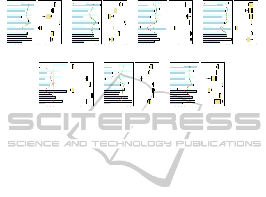
Figure 4 summarizes the results of classiﬁcation that

are represented by bars and lines at different color

scales. Each ﬁgure contains information about the

behavior of the geometric mean (red), the area un-

der the ROC curve (AUC) (green), sensitivity (color

light blue) and speciﬁcity (color light cyan). Each row

depict one of the class-balance strategies, sorted in

ascending order according to the strategy of balance:

oversampling (SMOTE), subsampling (SPSO), cost-

sensitive learning unused and using CuckooCost (CS,

CSCu,MC, MCCU) and Boosting (AdaBoost). On

the right side of the graph, it shows the dispersions of

classiﬁcation results obtained by each balance tech-

nique, exposed by means of boxplots.

Table 5 contains information concerning to data

complexity involved in the categories. This table

describes measurements that determine the overlap

and separability between classes (VOR, J4, Fisher),

and measurements of nonlinearity in the classiﬁers

(LOOerror1NN) contrasted with information of im-

balance degree for each dataset, this in order to obtain

AMethodologyforOptimizingtheCostMatrixinCostSensitiveLearningModelsappliedtoPredictionofMolecular

FunctionsinEmbryophytaPlants

SMOTE

SPSO

CSCu

MCCu

Ada

0.0 0.1 0.2 0.3 0.4 0.5 0.6 0.7 0.8 0.9 1.0

●

Sensitivity

Specificity

Geometric mean

AUC

Performance

● ●

●

0.50 0.55 0.60 0.65 0.70 0.75 0.80

Dispersion

(a) DNA binding.

SMOTE

SPSO

CSCu

MCCu

Ada

0.0 0.1 0.2 0.3 0.4 0.5 0.6 0.7 0.8 0.9 1.0

●

Sensitivity

Specificity

Geometric mean

AUC

Performance

●

●●

●

0.50 0.55 0.60 0.65 0.70 0.75 0.80 0.85

Dispersion

(b) Sequence-speciﬁc DNA binding -

transcription factor activity.

SMOTE

SPSO

CSCu

MCCu

Ada

0.0 0.1 0.2 0.3 0.4 0.5 0.6 0.7 0.8 0.9 1.0

●

Sensitivity

Specificity

Geometric mean

AUC

Performance

●

●●

●

●●

0.2 0.3 0.4 0.5 0.6

Dispersion

SMOTE

SPSO

CSCu

MCCu

Ada

0.0 0.1 0.2 0.3 0.4 0.5 0.6 0.7 0.8 0.9 1.0

●

Sensitivity

Specificity

Geometric mean

AUC

Performance

●

0.6 0.7 0.8 0.9

Dispersion

(d) Transporter activity.

SMOTE

SPSO

CSCu

MCCu

Ada

0.0 0.1 0.2 0.3 0.4 0.5 0.6 0.7 0.8 0.9 1.0

●

Sensitivity

Specificity

Geometric mean

AUC

Performance

●

0.2 0.3 0.4 0.5

Dispersion

(e) Hydrolase activity.

SMOTE

SPSO

CSCu

MCCu

Ada

0.0 0.1 0.2 0.3 0.4 0.5 0.6 0.7 0.8 0.9 1.0

●

Sensitivity

Specificity

Geometric mean

AUC

Performance

●

● ●

●

0.0 0.2 0.4 0.6 0.8

Dispersion

(f) Enzyme regulator activity.

SMOTE

SPSO

CSCu

MCCu

Ada

0.0 0.1 0.2 0.3 0.4 0.5 0.6 0.7 0.8 0.9 1.0

●

Sensitivity

Specificity

Geometric mean

AUC

Performance

●

●●

0.4 0.5 0.6 0.7 0.8

Dispersion

(g) Transcription regulator activity.

Figure 1: Molecular function prediction results.

information concerning to the difﬁculty to induce re-

liable learning models in each biclass problem. Mea-

sures such as Fisher discriminant ratio, J4 and tend

to be favorable as they increase in value, indicating

a greater separability, otherwise occurs VOR which

tends to be better as its value approaches zero, indicat-

ing a smaller area of overlap. According to the values

given in Table 5, The most complex space is the set

belonging to Hydrolase activity (GO 0016787), show-

ing a low value at J4 and VOR highest compared to

other classes. This fact is proved by the results ob-

tained for this class exhibited in Figure 1(a), Where

all techniques show poor performance balance. This

suggests that in this class will present a very poor rep-

resentation of the data. Also, if we look again the

values listed in the Table 5, The level of imbalance is

not as signiﬁcant as compared with the values of over-

lap between the data, which might lead to think that

data complexity can may deteriorate more severely

the learning process in protein prediction compared

with the class imbalance, only when level of overlap

and separability is to big compared with imbalance ra-

tio itself.Therefore, it is convenient to use complexity

measures as a complement to the level of imbalance

to be certain about the difﬁculty of the problem.

Despite the complexity, the best behavior for Hy-

drolase activity was obtained SPSO, with a value of

geometric mean (GM) and ROC area (AUC) just over

50% and very low dispersion in the prediction. How-

ever, the difference was very short compared to the

method based on cost sensitive learning using Cuck-

ooCost (CSCu). It is remarkable that in datasets with

higher imbalance between categories such as Enzyme

regulator activity and Sequence-speciﬁc DNA bind-

ing transcription factor activity (GO 0030234 and GO

0003700), CSCu obtained a considerable superior-

ity over the techniques compared, in fact, its perfor-

mance overcomes in ﬁve of the seven categories (GO

0030234, GO 0003700, GO 0003677, GO 0030528

and GO 0005215), and the remaining 2 sets (GO

0016787 and GO 0003824) was one of the highest

performing techniques in his prediction, as can be

seen in Table 6

On the other hand, AdaBoost and SMOTE obtain

the worst prediction results, especially in Hidrolase

activity, Enzyme regulator activity and Transcription

regulator activity (GO 0016787, 0030234 and GO

0030528). From these results we conclude that in the

presence of sets with high overlap, oversampling can

be conterproductive, due to there exist a high proba-

bility of adding extra noise in the training set when

synthetic samples are adding, interfering with the in-

duction of a reliable model for prediction of molecu-

lar functions. In case of AdaBoost, the high overlap

can decrease considerably the generalization capabil-

ity of the classiﬁers used by this technique, when it is

forced to be rather complex decision boundaries.

An important fact shown in Figure 4 and the over-

all results of the Table 6, is the effect of CuckooCost

in methods based on cost sensitive learning over their

performance (CS,MC,CSCu,MCCu). Clearly shows

a substantial improvement in MetaCost and cost sen-

sitive learning in overall performance (increased GM

and AUC), as well as the reliability of the results by

decreasing the classiﬁcation dispersion in every cate-

gory. Although MetaCost follows the same trend of

improvement when using CuckooCost in transporter

activity (GO 0005215), it is seen a slight increase in

BIOINFORMATICS2013-InternationalConferenceonBioinformaticsModels,MethodsandAlgorithms

Table 5: Table of data complexity measurements in the datasets.

Categories Fisher Discriminant Ratio VOR J4 LOO error 1NN (%) Imbalance

GO 0003677 1,162564308 1,518414e-45 366,65 42 1:7,68

GO 0003700 1,258898151 8,325292e-43 153,09 54,7 1:10,76

GO 0003824 0,095424389 1,503915e-39 114,67 41,3 1:2,74

GO 0005215 1,275657636 1,974715e-67 3045,37 19,4 1:8,26

GO 0016787 0,004254501 6,654359e-07 -0,472 53,9 1:4,63

GO 0030234 0,265168845 1,247835e-26 14,712 79,3 1:23,87

GO 0030528 0,954652410 1,125151e-37 255,43 37,6 1:7,22

Table 6: Table of AUC and GM.

Categories SMOTE SPSO CS CSCu MC MCCu Ada

AUC GM AUC GM AUC GM AUC GM AUC GM AUC GM AUC GM

GO 0003677 0,693 0,668 0,708 0,707 0,615 0,519 0,788 0,786 0,684 0,659 0,718 0,713 0,766 0,747

GO 0003700 0,654 0,599 0,721 0,721 0,679 0,629 0,821 0,817 0,617 0,566 0,668 0,655 0,773 0,744

GO 0003824 0,664 0,658 0,667 0,667 0,53 0,292 0,655 0,651 0,618 0,592 0,661 0,654 0,599 0,536

GO 0005215 0,778 0,752 0,811 0,81 0,643 0,562 0,829 0,823 0,803 0,788 0,839 0,835 0,812 0,766

GO 0016787 0,505 0,405 0,516 0,513 0,497 0,188 0,504 0,49 0,499 0,395 0,499 0,443 0,485 0,128

GO 0030234 0,568 0,429 0,663 0,642 0,618 0,613 0,699 0,686 0,515 0,205 0,617 0,518 0,675 0,502

GO 0030528 0,659 0,621 0,717 0,714 0,595 0,493 0,763 0,762 0,68 0,662 0,676 0,66 0,723 0,691

Total 0,646 0,59 0,686 0,682 0,596 0,47 0,723 0,717 0,63 0,552 0,668 0,64 0,69 0,588

the variance of the result. This may be due to an ap-

propriate number of iterations for MetaCost (10 iter-

ations) was not taken. MetaCost use resampling via

Bootstrap, taking a portion of the training set to cre-

ate a subset in each iteration, then each subset is taken

by a number of base classiﬁers equal to the number

of iterations for the algorithm selected and the ﬁnal

classiﬁcation decision is taken in committee by a vote

of each classiﬁer. When the number of iterations in

MetaCost is not adequate and additionally the dataset

have a substantial degree of imbalance, as it is in this

case, the number of samples of interest, i.e the sam-

ples belonging to this category used for each base

classiﬁer could not be enough.

In all categories, there exist cases where some bal-

ance techniques present very similar values of GM

compared with their AUC values, mainly in SPSO

and CSCu. It observes that occurs particularly when

the numeric difference between sensitivity and speci-

ﬁcity is small, i.e, the numeric values of sensitivity

and speciﬁcity are to close among them. This fact

can be corroborated with the relative sensitivity val-

ues (RS) (Su and Hsiao, 2007), exposed in Table 7.

Table 7: Table of relative sensitivity.

Categories SMOTE SPSO CS CSCu MC MCCu Ada

GO 0003677 0,582 0,996 3,301 1,119 0,582 0,796 1,572

GO 0003700 0,427 1,067 2,185 1,217 0,433 0,676 1,701

GO 0003824 0,766 0,973 11,057 0,803 0,555 0,755 0,406

GO 0005215 0,593 1,002 2,885 0,8 0,688 0,842 0,762

GO 0016787 0,251 1,234 25,892 0,614 0,241 0,371 0,017

GO 0030234 0,208 1,652 0,783 0,677 0,044 0,297 0,269

GO 0030528 0,503 1,203 3,541 1,126 0,631 0,651 1,824

As it can seen, SPSO and CSCu are the techniques

with less bias in their classiﬁcations, with values more

close to one. The above indicates that precisely these

two classiﬁers try to obtain an equilibrium between

sensibility and speciﬁcity values, fact that is shown

with the points in Figure 4 where AUC = GM. Con-

trary to popular belief, SMOTE tends to be very spe-

ciﬁc, although sampling techniques try to become

more sensitive to increase distribution of samples on

category with lower representation. it is noteworthy

that both CS and MC obtained a quite substantial im-

provement when they use CuckooCost to optimize

their parameters, initially CS was to sensitive but it

had a small s peciﬁcity, contrary case to MC, that it

had a big speciﬁcity. When CuckooCost was used,

both strategies were proximal to one, specially in CS.

6 CONCLUSIONS AND FUTURE

WORK

A method to optimize the free parameters associated

to cost sensitive learning, applied to prediction of

molecular functions in embryophita plants was pro-

posed, with the purpose of having direct control over

sensitivity and speciﬁcity of the classiﬁcation (related

to the costs involved misclassifying samples belong-

ing to each category). The optimization is proposed

over the elements of the cost matrix, whose tuning

was adapted on elements outside the main diagonal,

building the cost ratio. The variation of the cost ratio,

along with the classiﬁcation parameters were used as

hyperparameters in the optimization problem, since

the metric intrinsically modify the ﬁtness function. To

this purpose, a metaheuristic optimization technique

called Cuckoo Search was used. The methodology

AMethodologyforOptimizingtheCostMatrixinCostSensitiveLearningModelsappliedtoPredictionofMolecular

FunctionsinEmbryophytaPlants

takes as ﬁtness function the maximization of adjusted

geometric mean (AGM) (Batuwita and Palade, 2009).

This work demonstrated that the use of models based

on cost sensitivity learning are very competitive and

reliable, and even superior to other balance techniques

in the state of the art, specially in applications related

to bioinformatics. As future work, the use of other

metrics as ﬁtness function for improving the costs

associated with the classiﬁcation, such as ROC area

(AUC), Geometric Mean (GM), Mathews Correlation

Coefﬁcient (MCC) or another relationships between

sensitivity and speciﬁcity can be considered.

ACKNOWLEDGEMENTS

This work was partially funded by the Research

ofﬁce (DIMA) at the Universidad Nacional de

Colombia at Manizales and the Colombian National

Research Centre (COLCIENCIAS) through grant

No.111952128388 and the ”jovenes investigadores e

innovadores - 2010 Virginia Gutierrez de Pineda” fel-

lowship.

REFERENCES

Ashburner, M., Ball, C., Blake, J., Botstein, D., Butler, H.,

Cherry, J., Davis, A., Dolinski, K., Dwight, S., Eppig,

J., et al. (2000). Gene ontology: tool for the uniﬁca-

tion of biology. Nature genetics, 25(1):25.

Basu, M. (2006). Data complexity in pattern recognition.

Springer-Verlag New York Inc.

Batuwita, R. and Palade, V. (2009). A new performance

measure for class imbalance learning. application to

bioinformatics problems. In Machine Learning and

Applications, 2009. ICMLA’09. International Confer-

ence on, pages 545–550. IEEE.

Chawla, N., Bowyer, K., Hall, L., and Kegelmeyer, W.

(2002). Smote: synthetic minority over-sampling

technique. Journal of Artiﬁcial Intelligence Research.,

16:321– 357.

Ding, Z. (2011). Diversiﬁed ensemble classiﬁers for highly

imbalanced data learning and its application in bioin-

formatics. PhD thesis, GEORGIA STATE UNIVER-

SITY.

Domingos, P. (1999). Metacost: A general method for

making classiﬁers cost-sensitive. In Proceedings of

the ﬁfth ACM SIGKDD international conference on

Knowledge discovery and data mining, pages 155–

164. ACM.

Elkan, C. (2001). The foundations of cost-sensitive learn-

ing. In International Joint Conference on Artiﬁcial In-

telligence, volume 17, pages 973–978. LAWRENCE

ERLBAUM ASSOCIATES LTD.

Frishman, D., Argos, P., et al. (1997). Seventy-ﬁve percent

accuracy in protein secondary structure prediction.

Proteins-Structure Function and Genetics, 27(3):329–

335.

Garc

ıa-L

opez, S., Jaramillo-Garz

on, J. A., Higuita-

asquez, J., and Castellanos-Dom

ınguez., C. (2012).

Wrapper and ﬁlter metrics for pso-based class bal-

ance applied to protein subcellular localization. In

BIOSTEC-BIOINFORMATICS 2012.

Grzymala-Busse, J., Stefanowski, J., and Wilk, S. (2005).

A comparison of two approaches to data mining from

imbalanced data. Journal of Intelligent Manufactur-

ing, 16(6):565–573.

He, H. and Garcia, E. (2009). Learning from imbalanced

data. Knowledge and Data Engineering, IEEE Trans-

actions on, 21(9):1263–1284.

Jain, E., Bairoch, A., Duvaud, S., Phan, I., Redaschi, N.,

Suzek, B., Martin, M., McGarvey, P., and Gasteiger,

E. (2009). Infrastructure for the life sciences: de-

sign and implementation of the uniprot website. BMC

bioinformatics, 10(1):136.

Larra

naga, P., Calvo, B., Santana, R., Bielza, C., Galdiano,

J., Inza, I., Lozano, J., Arma

nanzas, R., Santaf

e, G.,

erez, A., et al. (2006). Machine learning in bioinfor-

matics. Brieﬁngs in bioinformatics, 7(1):86–112.

Liu, X. and Zhou, Z. (2006). The inﬂuence of class im-

balance on cost-sensitive learning: an empirical study.

In Data Mining, 2006. ICDM’06. Sixth International

Conference on, pages 970–974. IEEE.

Liu, X. and Zhou, Z. (2012). Towards cost-sensitive learn-

ing for real-world applications. New Frontiers in Ap-

plied Data Mining, pages 494–505.

Polikar, R. (2006). Ensemble based systems in deci-

sion making. Circuits and Systems Magazine, IEEE,

6(3):21–45.

Schapire, R. (1999). A brief introduction to boosting. In

International Joint Conference on Artiﬁcial Intelli-

gence, volume 16, pages 1401–1406. LAWRENCE

ERLBAUM ASSOCIATES LTD.

Sonnenburg, S., Schweikert, G., Philips, P., Behr, J., and

atsch, G. (2007). Accurate splice site prediction us-

ing support vector machines. BMC bioinformatics,

8(Suppl 10):S7.

Su, C. and Hsiao, Y. (2007). An evaluation of the robustness

of mts for imbalanced data. Knowledge and Data En-

gineering, IEEE Transactions on, 19(10):1321–1332.

Valian, E., Mohanna, E., and Tavakoli, S. (2011). Im-

proved cuckoo search algorithm for global optimiza-

tion. Int. J. Communications and Information Tech-

nology, 1(1):31–44.

Yang, P., Xu, L., Zhou, B., Zhang, Z., and Zomaya, A.

(2009). A particle swarm based hybrid system for

imbalanced medical data sampling. BMC genomics,

10(Suppl 3):S34.

Yu, L. and Liu, H. (2004). Efﬁcient feature selection via

analysis of relevance and redundancy. The Journal of

Machine Learning Research, 5:1205–1224.

BIOINFORMATICS2013-InternationalConferenceonBioinformaticsModels,MethodsandAlgorithms