
Regularized Least Squares Applied to Heartbeat Classification using
Transform-based and RR Intervals Features
Hamza Baali, Rini Akmeliawati and Momoh J. E. Salami
International Islamic University Malaysia (IIUM), Department of Mechatronics Engineering
Jalan Gombak, 53100 Kuala Lumpur, Malaysia
Keywords: Arrhythmia Classification, Aami, ECG, PVC, RLSC, Transformation.
Abstract: An algorithm for arrhythmia classification is presented with emphasis on the discrimination between normal
and premature ventricular contraction (PVC) conditions. We derived new features from the transformed
ECG signal resulting from the linear predictive analysis of the ECG heartbeats and from the LPC filter
impulse response matrix. These features in conjunction with the residual error energy and RR-intervals are
fed into the Regularized Least Squares Classifier (RLSC) with radial basis kernel. The proposed features
show an acceptable separation capability between the two classes. Two scenarios are investigated using
selected records taken from the MIT-Arrhythmia database namely, intra-patient and inter-patient
classification. The achieved results are 98.18 sensitivity and 99.02 specificity in average for the first
scenario (intra-patient) and 95.18 sensitivity and 96.92 specificity in average for the second scenario (inter-
patient).
1 INTRODUCTION
Electrocardiogram (ECG) is a crucial diagnostic tool
for monitoring cardiac activities. Abnormalities in
both electrical generation and conduction at different
levels in the heart are reflected on the ECG as
deviations from the normal heart rhythm. The term
Arrhythmia is used to refer to these deviations. In
spite of many research efforts devoted to automatic
arrhythmia monitoring, none of the developed
methods are completely satisfactory. The challenge
is due to the variations in the morphology of ECG
heartbeats which exhibit the same type of
arrhythmias within and across patients. Moreover, in
many cases heartbeats with different types of
arrhythmias have similar morphology and frequency
content (Osowski and Linh, 2001). These intra-class
variations and inter-class similarities make it
difficult to extract discriminative features from the
time series of the heartbeats. To overcome this
problem many authors have proposed Patient-
Adapting Heartbeat Classifiers whereby a manual
labelling of heartbeats from all new patients is
needed and the classifier is adapted accordingly
(De Chazal and Reilly,2006., Hu et al.,1997,
Lagerholm et al., 2000). Though these approaches
considerably improve the classifier performances,
they do not seem practical, especially in developing
countries, due to the cost of acquiring trained
physicists who are able to label the data for each
new patient. The ultimate aim in this research area is
the development of a classifier that performs well on
the unseen data without “assistance” from physicists.
This study investigates the use of a Regularised
Least Squares Classifier for the classification of
normal (N) and abnormal premature ventricular
contraction (PVC) conditions.
Unlike normal beats which originate from the
sinoatrial (SA) node, PVC beats originate from the
ventricles and are characterised by the absence of
the P wave and a large QRS complex as illustrated
in Figure 1. Their presence in an ECG record
becomes clinically significant only if their frequency
of occurrence exceeds six beats per minutes.
Examples of these complex PVCs include, bigeminy
(every other beat is a PVC), multifocal (varied
shapes and forms of the PVCs) and coupling (two
PVCs occur back to back). These complex PVCs
could degenerate into serious ventricular
arrhythmias such as ventricular tachycardia (Sigg
et al., 2005). Therefore, many lives could be saved if
these beats are detected early-on and accurately. To
achieve good classification results, the set of input
features as well as the classifier are crucial.
164
Baali H., Akmeliawati R. and J. E. Salami M..
Regularized Least Squares Applied to Heartbeat Classification using Transform-based and RR Intervals Features.
DOI: 10.5220/0004242101640170
In Proceedings of the International Conference on Bioinformatics Models, Methods and Algorithms (BIOINFORMATICS-2013), pages 164-170
ISBN: 978-989-8565-35-8
Copyright
c
2013 SCITEPRESS (Science and Technology Publications, Lda.)

Figure 1: Premature ventricular contractions with different
shapes.
Autoregressive (AR) modeling has been adopted for
ECG compression and monitoring (Ge et al.,2002.,
Ham and Han, 1996., Lin and Chang, 1989). The
ECG signal can be reconstructed using the residual
error and the linear prediction coefficients (LPC)
using the synthesis filter. Though the representation
and the use of the LPC filter coefficients as features
have been well studied and understood, the
extraction of relevant features from the residual error
should receive much more emphasis as suggested by
(Lin and Chang, 1989).
In this paper, a new set of features extracted from
the impulse response matrix of the LPC filter and the
transformed ECG signal is proposed. Using this
approach, each ECG period is orthogonally
transformed into a new domain where only few
coefficients contain most of the signal information.
The extracted features are fed into the classifier in
conjunction with some commonly used features
including the residual error energy and RR intervals
(Ge et al., 2002., De Chazal et al., 2004., Lannoy et
al., 2011). The performances of the proposed
algorithm are evaluated on clinical ECG data
selected from the MIT-BIH arrhythmia database.
The database is the most frequently used database
for arrhythmia classification.
The paper is organised as follows, ECG filtering
is presented in section 2.1, while Autoregressive
modeling of the ECG signal is discussed in section
2.2. Feature extraction is examined in section 2.3,
Regularised least squares classifier is presented in
section 2.4. Results and a discussion of the
performances of the proposed algorithm are given in
section 3 and section 4 holds the conclusions.
2 METHODS
2.1 ECG Filtering
The raw ECG signal is usually contaminated with
different types of noise (eg., Baseline wander, power
line interference, and high-frequency noise). ECG
filtering is aimed at improving the signal to noise
ratio (SNR) by removing the noise (Clifford et
al.,2006.).
In order to remove the power line interference, a
second order notch-filter centred on
60Hz
with a bandwidth ΔF 3Hz is first applied to the
ECG signal. The transfer function of the filter is
given by:
2cos
12cos
,
(1)
where
|
|
|
|
;
2
;1
ΔF
;
360.
The parameter controls the spectral width and
depth of the filter.
Afterwards, the baseline wander is removed from
the ECG signal by cascading two median filters of
lengths 108 (0.3
) and 216 (0.6
) samples,
respectively. The first filter is aimed at removing the
QRS complexes and the P-waves from the ECG,
while the second filters the T waves. The output of
the second filter is subtracted from the original ECG
signal to obtain a corrected baseline ECG. Finally,
the high frequency noise is filtered by biorthogonal
wavelet, where the first approximation is kept as
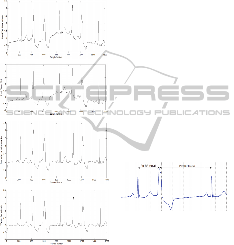
filtered ECG.A step by step demonstration of ECG
filtering is given Figure 2.
2.2 Autoregressive Modeling of ECG
AR modeling consists of estimating the value of the
current sample as a linear combination of P past
samples, that is,
,
(2)
where
is the predicted signal,
are the
LPCs,
is the i-th previous sample of the
ECG signal and P is the model order.
The prediction coefficients may be found by
minimizing the sum-of-squared error (SSE) between
the actual sample and the predicted one with respect
to the LPC coefficients as given bellow:
∑
∑
∑
0
(3)
The autocorrelation method is computationally more
efficient and the filter is guaranteed to be stable
(Makhoul, 1975). The original signal can be
reconstructed using the residual error and the LPCs
using the synthesis filter, that is,
RegularizedLeastSquaresAppliedtoHeartbeatClassificationusingTransform-basedandRRIntervalsFeatures
165
,1
(4)
(a)
(b)
(c)
(d)
Figure 2: ECG Filtering, a-Raw ECG taken from record
208,b-Notch filtered ECG ,c-baseline wander removal
using 2 median filters, d- bior3.3 wavelet first
approximation ECG.
where is the synthesis filter impulse response
and is the size of the ECG period.
A fourth-order LPC analysis is performed on each
ECG heartbeat belonging to one of the two classes
considered in this study (Ge et al,2002). We
consider that each heartbeat starts from the midpoint
between the R-peak of the given heartbeat and the
R-peak of the previous heartbeat and ends on the
midpoint between the R-peak of the current
heartbeat and the R-peak of the following heartbeat.
We use the heartbeat fiducial point times provided
with the MIT-BIH arrhythmia database to locate the
R-peaks (Mark and Moody, 1997).
2.3 ECG Features
As mentioned in Section 1, the set of features plays a
vital role in achieving good classification results. To
this end, each ECG heartbeat is transformed into a
feature vector. In this section, we use some features
that have been successfully used in previous studies
for ECG monitoring and we propose new set of
features to explore more information from the ECG
data.
2.3.1 RR-Interval Features
The RR-interval is the interval between two
consecutive R-peaks. Two RR-intervals are
measured, namely the RR-interval between the
actual heartbeat and the preceding heartbeat (Pre-RR
interval) and the RR-interval between the actual
heartbeat and the subsequent heartbeat (Post-RR
interval) as shown in Figure 3.
Figure 3: Pre-RR and Post-RR intervals.
2.3.2 Residual Error Energy
Residual error energy (
) is a time-domain
measurement that characterises the performance of
the prediction, it is defined as:
(5)
2.3.3 Transformation based Features
An interesting framework for an accurate
representation of the excitation signal applied to
speech signal was initiated by (Atal, 1989), and this
was later investigated and further developed by our
BIOINFORMATICS2013-InternationalConferenceonBioinformaticsModels,MethodsandAlgorithms
166
group for ECG compression in (Baali, Salami,
Akmeliawati and Aibinu, 2011) and for ECG period
normalization in (Baali, Akmeliawati, Salami,
Aibinu and Gani, 2011). The representation in
question is subsequently described and adopted for
features extraction.
Equation (4) can be expressed in matrix as:
,
(6)
whereis1column vector in which its entries
represented by the ECG samples and is an 1
column vector of the residual error. is the
impulse response matrix of the synthesis filter (also
called LPC filter), its entries are completely
determined by the linear prediction coefficients, is
a lower triangular and Toeplitz matrix.
1
1
⋮
.
1
0
1
⋮
.
2
⋯
⋱
⋱
.
.
.
.
.
.
.
0
0
⋮
.
1
,
(7)
Applying the singular values decomposition (SVD)
to gives:
,
(8)
where and are orthogonal matrices, and
is a real valued diagonal matrix of the
singular values of .
The SVD domain representations of and are
given by and respectively, where
and
.
Therefore;
(9)
From (9) each component of the residual signal ()
is projected onto the right singular vectors of the
matrix H and then weighted by the corresponding
singular value. Since the singular values are always
arranged in a descending order, one can expect that
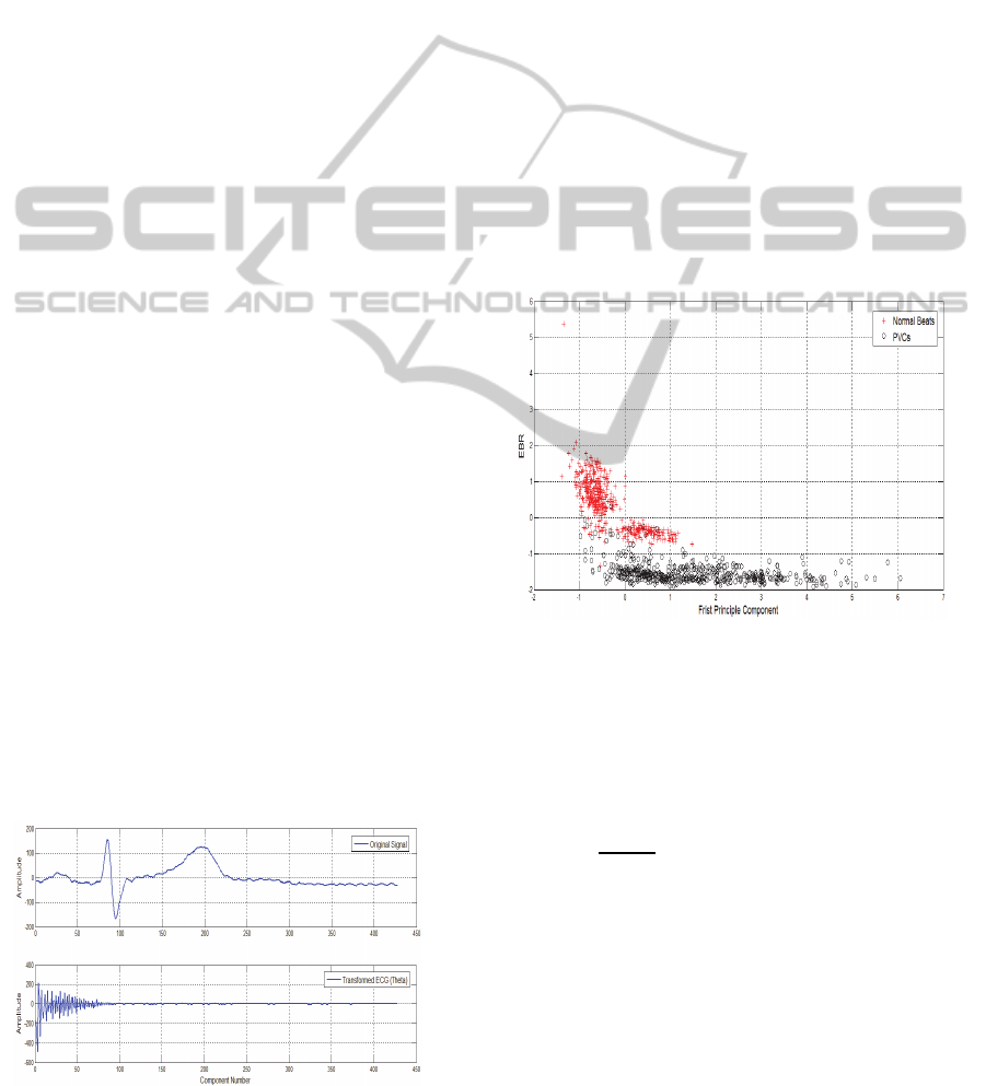
the transformed ECG signal () is decaying as seen
in Figure 4.
Figure 4: Normal sinus beat and transformed ECG.
From this transformation two features may be
introduced:
1- The ratio between the number of elements
containing 90% of the total energy of the
transformed ECG () and the length of the ECG
heartbeat (i.e., Energy Based Ratio (EBR) .The
energy of the ECG waveform and the transformed
ECG is the same since the mapping
is
isometric.
2- The largest singular value of the impulse
response matrix.
For instance, Figure 5 represents a two-dimensional
feature space of normal (red ‘+’) and PVC (black
‘o’) beats randomly taken from three different
patients with identification numbers 116, 208 and
210. The first feature corresponds to the first
principle component of the impulse response matrix
H, while the second represents the EBR. The cluster
plot shows that the newly introduced features have a
good discrimination capability between the normal
(NOR) and PVC beats.
Figure 5: Two-dimensional feature vectors of normal (red
‘+’) and PVC beats (black ‘o’).
2.4 Feature Normalization
A linear method is used to normalize the features to
zero mean and unit variance, such that:
̅
, 1,2,…….,
(10)
where
is the normalised value, ̅ and are
respectively the mean value and standard deviation.
2.5 RLS Classifier
The use of Regularized least squares (RLS) is
considered in this paper, where the aim is to build a
function (i.e., a learning model) using a set of
training points that accurately predicts the class to
RegularizedLeastSquaresAppliedtoHeartbeatClassificationusingTransform-basedandRRIntervalsFeatures
167

which the test points belong (i.e., unseen examples).
The RLS is a special case of the Tikhonov
regularization problem which is mathematically
stated as (Rifkin, 2002).
min
∈
1
ℓ
,
ℓ
λ
‖
‖
,
(11)
where is the loss function, λ is the regularization
parameter (λ∈
).
‖
‖
is the norm of
measured in a Reproducing Hilbert space defined by
the kernel K. The square loss function is given by :
,
,
(12)
where
denotes the d-dim feature vector of the ith
training point and
∈
1,1
gives the binary
outcome, for1,…,ℓ (with ℓ is the number of
training points).
The Representer Theorem (Rifkin, 2002) states that
for some
the solution
∗
of (11) has the form:
∗
K
,
ℓ
∈
(13)
There is a wide range of possible kernel functions
that might be used, however, in this paper the linear
kernel is chosen, that is,
K
,
(14)
The kernel function measures the similarity between
two feature vectors. The selection of the linear
kernel is justified by the fact that it allows a lower
computational complexity compared to other kernels
(Rifkin and Lippert, 2007).
The norm of is given by :
‖
‖
. ∈
ℓ
,∈
ℓℓ
,
(15)
where is the square positive semidefinite training
kernel matrix with elements :
,
K
,
, for ∶ 1,…,ℓand 1,…,ℓ.
By using (12), (13) and (15), the Tikhonov
regularization problem can be rewritten as:
min
∈
ℓ
1
2ℓ
λ
2
,
∈
ℓ
with coordinates
.
(16)
The problem is brought forward to find the ℓ-dim
weight vector where the minimization of (16) with
respect to has the closed form solution:
λ
ℓ
∈
ℓℓ
is the identity matrix.
(17)
Once the weight vector is found, the
determination of class membership of a test point
is possible. Thus,
∗
K
,
ℓ
.
(18)
In binary classification, the label (or class) of
is determined by the sign of
∗
.
2.5.1 Tuning the Regularization
Parameter
The weight vector is a function of the
regularization parameter λ. Rifkin and Lippert,
(2007) proposed an elegant way of tuning λ by
rewriting (17) using the eigendecomposition of the
kernel matrix .
Let
and
, then,
λℓ
,
(19)
where
λ
,…,λ
ℓ
. Writing in the form
given by (18) allows one to vary λ between the
minimum and maximum eigenvalues of
efficiently. Note that the matrix
λℓ is
diagonal, hence;
λ
.
3 RESULTS AND DISCUSSION
The performance of the proposed algorithm is
evaluated on clinical ECG data selected from the
MIT-BIH arrhythmia database. The database is the
most frequently used database for arrhythmia
classification. It contains 48 half hour recordings of
two-channel ambulatory ECG filtered from 0.1 to
100 Hz then sampled at 360 Hz (Mark and Moody,
1997). The data set used in this study is collected
from six patients with large number of PVCs
namely, records with identification numbers 116,
208, 210, 228 and 233. The selected data set consists
of 12245 normal beats and 2882 PVCs.
Each of the extracted heartbeats is transformed into
a five-dimensional feature vector (Residual error
energy, the largest singular value of H, EBR and 2
RR-intervals).
Two metrics are used to assess the performance of
the proposed algorithm, namely Sensitivity (Se) and
specificity (Sp). Sensitivity is the fraction of PVCs
that are correctly classified, and is given by:
Se = TP / (TP + FN)
BIOINFORMATICS2013-InternationalConferenceonBioinformaticsModels,MethodsandAlgorithms
168

Specificity is the fraction of normal beats that are
correctly classified, and is given by:
Sp = TN/ (TN + FP)
TP, FP, FN and TN stand for true positives , false
positives , false negatives and true negatives,
respectively.
Two different tests are carried out:
First Scenario:
The whole data set is randomly split into two non-
overlapped parts: a training set and a test set. The
training set is used to tune the regularization and the
kernel parameters while the test set is held-out for
validation. This approach is referred to as “intra-
patient” classification since the training set contains
samples from all patients.
We increase the number of training points taken
from each class from initially 250 to 500 then to
750. We run each experiment 5 times. The average
values of specificity (Av Sp) and sensitivity (Av Se)
are shown in Table.1.
Table 1 : Intra-patient classification performances.
Number of
Training points
per class
Number of Test
points
Av.Se Av.Sp
250 14627 97.67 098.77
500 14127 97.69 99.14
750 13627 98.18 99.02
Second Scenario:
In this scenario, the training points are randomly
extracted from records 116, 208 and 210 and then
tested on the unseen data which are composed from
records 221,228 and 233. This approach is referred
to as “inter-patient” classification. Similar to the
first scenario, each experiment is run 5 times. Table
2 summarises the results.
Table 2 : Inter-patient classification performances.
Number of
Training points
per class
Number of
Test points
Av. Se Av.Sp
250 7743 92.54 92.69
500 7743 93.79 92.52
750 7743 95.18 96.92
In the first scenario we notice that the increase of the
number of training points does not considerably
improve the performances of the classifier (When
the number of training points was increased by
150%, the improvement of performances was less
that 1% in both metrics ). The best results achieved
were 98.18 sensitivity and 99.02 specificity.
On the other hand, the second scenario has
demonstrated the stability of the proposed features
where only a slight decrease (less than 3%) in
performances was recorded when compared to the
first scenario. In addition, we notice that unlike the
first scenario, the increase of the training points
improves the performances by around 3% in both
metrics.
In order to assess the merit of the proposed
classification scheme, Table 3 depicts the overall
classification performance of the proposed RLSC
along with some benchmark methods. Bortolan,
Jekova and Christov (2005) investigated four
classification techniques namely, neural networks
(NN), K-nearest-neighbour (KNN), linear
discriminant (LD) and Fuzzy logic using 26
morphology features and patient adapting (PA)
strategy. The best results were achieved by NN
classifier. Mai1 and Khalil (2011), on the other
hand, adopted PA strategy to discriminate between
normal and PVC conditions where Cardioid loop
coordinates were extracted from the ECG heartbeats
and serve as input to the NN classifier. Meanwhile,
Shyu, Wu, and Hu (2004) implemented a Fuzzy-
Neural networks (FNN) classifier with features
extracted from wavelet decomposition of the ECG
signal and by adopting inter-patient scenario.
The achieved results were very encouraging as the
performances obtained were comparable to many
state-of-the-art inter-patients algorithms.
Table 3: Comparison of the proposed RLSC with
benchmark methods.
Classification
strategy
Training
strategy
Se Sp
NN [19]
NN [20]
FNN [21]
PA
PA
Inter-patient
95.8
97.34
99.86
98.3
98.62
99.79
KNN [19] PA 91.3 98.7
DA[19] PA 97.0 94.4
Fuzzy logic [19] PA 92.8 98.4
RLSQ (proposed) Inter-patient 95.18 96.92
RLSQ (proposed) Intra-patient 98.18 99.02
4 CONCLUSIONS
The main contribution of this paper is
thedevelopment of stable features for Arrhythmia
classification. The performances of the proposed
features are appreciated when implemented with
RLS classifier and validated on selected records
from the MIT-Arrhythmia database. When the
linear prediction coefficients are used with the
aforementioned features, the classifier achieved
lower performance results. For instance, the average
RegularizedLeastSquaresAppliedtoHeartbeatClassificationusingTransform-basedandRRIntervalsFeatures
169

specificity and sensitivity were respectively, 98.43
and 97.28 in the first scenario. Further work should
focus on the extraction of more features from the
residual signal.
ACKNOWLEDGEMENTS
This work was supported by the ministry of higher
education (MOHE) of Malaysia under the
fundamental research grant scheme FRGS.
REFERENCES
Osowski, S., Linh, T. L., 2001. ECG beat recognition
using fuzzy hybrid neural network. IEEE Trans.
Biomed. Eng. 48 (11), 1265-1271.
De Chazal, P., Reilly, R. B.,2006. A Patient-Adapting
Heartbeat Classifier Using ECG Morphology and
Heartbeat Interval Features. IEEE Trans. Biomed. Eng.
53 (12), 2535-2543.
Hu,Y. H., Palreddy, S., Tompkins, W. J .,1997. A patient-
adaptable ECG beat classifier using a mixture of
experts approach. IEEE Trans. Biomed. Eng. 44 (9),
891-900.
Lagerholm, M., Peterson, C., Braccini, G., Edenbrandt, L.,
Sornmo,L.,2000. Clustering ECG complexes using
hermite functions and self-organizing maps. IEEE
Trans. Biomed. Eng. 47 (7), 338-348.
Sigg, D. C., Iaizzo, P. A., Xiao, Y F, He, B.,2010. Cardiac
Electrophysiology Methods and Models.: Springer.
Ge D., Srinivasan, N., Krishnan,S M.,2002. Cardiac
arrhythmia classification using autoregressive
modeling. Biomed Eng Online. 1 (5), 1-12.
Ham, F. M., Han, S.,1996. Classification of cardiac
arrhythmias using fuzzy ARTMAP. IEEE Trans.
Biomed. Eng. 43 (4), 425-430.
Lin, K. P., Chang, W. H.,1989. QRS feature extraction
using linear prediction. IEEE Trans. Biomed. Eng. 35
(10), 1050-055.
De Chazal, P., O’Dwyer, M., Reilly, R .,2004. Automatic
classification of heartbeats using ECG morphology
and heartbeat interval features. IEEE Trans. Biomed.
Eng. 51 (7), 1196-1206.
Lannoy, G. D., François, D., Delbeke, J.,Verleysen, M.,
2011. Weighted SVMs and Feature Relevance
Assessment in Supervised Heart Beat
Classification. Commun. Comput. Inf. Sci. 127, 212-
223.
Clifford, G D., Azuaje, F., McSharry, P., 2006. Advanced
Methods And Tools for ECG Data Analysis: Artech
House, Inc., Norwood.
Makhoul, J.,1975. Linear prediction: A tutorial
review. Proceedings of the IEEE. 63 (4), 561-580 .
Mark, R., Moody,G. (1997). MIT-BIHArrhythmia
Database. Available: http://ecg.mit.edu/dbinfo.html.
Last accessed june 2012.
Atal,B .,1989. A model of LPC excitation in terms of
eigenvectors of the autocorrelation of the impulse
response of the LPC filter. ICASSP. 1, 45-48.
Baali, H., Salami, M. J. E ., Akmeliawati, R., Aibinu, A M
. (2011). Analysis of the ECG Signal using SVD-
Based Parametric Modelling Technique. International
Symposium on Electronic Design, Test and
Application ., 180-184.
Baali, H., Akmeliawati, R., Salami, M. J. E., Aibinu, M.
A., Gani A. (2011). Transform Based Approach for
ECG Period Normalization. Computing in Cardiology.
38, 533-536.
Rifkin R. M.,2002. Everything Old Is New Again: A Fresh
Look at Historical Approaches to Machine
Learning. Phd Thesis, Massachusetts Institute of
Technology
.
Rifkin, R. M., Lippert, R. A. 2007. Notes on Regularized
Least Squares.Computer Science and Artificial
Intelligence Laboratory Technical Report. 1-8.
Bortolan, G., Jekova , I., Christov, I., 2005. Comparison of
Four Methods for Premature Ventricular Contraction
and Normal Beat Clustering.Computing in Cardiology.
31, 921-924.
Mai,V., Khalil, I.,2011. A Cardioid Based Technique to
Identify Premature Ventricular Contractions.
Computing in Cardiology. 38 , 673-676.
Shyu, L. Y., Wu, Y. H ., Hu, W.,2004. Using wavelet
transform and fuzzy neural network for VPC detection
from the Holter ECG. IEEE Trans. Biomed. Eng. 51
(7), 1269-1273.
BIOINFORMATICS2013-InternationalConferenceonBioinformaticsModels,MethodsandAlgorithms
170
