Musculoskeletal System Modelling

Interpolation Method for Muscle Deformation

Jana Hájková and Josef Kohout

Department of Computer Science and Engineering, University of West Bohemia, Plzeň, Czech Republic

Keywords: Deformation, Muscle Modelling, Interpolation, Musculoskeletal Model, Action Line, Mesh Skinning.

Abstract: In this paper we present an interpolation method that was derived from the muscle deformation algorithm

computed on the gradient domain deformation technique. The method uses linear constraints to preserve the

local shape of the muscle and the non-linear volume constraints to preserve the volume of the mesh. The

Gauss-Newton method with Lagrange multipliers is used as the main computation algorithm and the inter-

polation approach serves especially to smooth up deformation steps. Thanks to the interpolation of main

bones movement positions by several temporally interpositions, the large distances are optimized and the

muscles of the musculoskeletal model are deformed in a more realistic way. The method was implemented

in C++ language, using VTK framework and was integrated into the human body framework. Despite the

fact that the current implementation is not optimised, all muscles tested were processed in a few minutes on

commodity hardware, which is much faster in comparison with the traditional FEM approaches.

1 INTRODUCTION

The musculoskeletal modelling and simulation is an

important step in predicting and personalizing the

treatment for the osteoporosis patients. In the

VPHOP project (VPHOP, 2012), we aim, therefore,

at creating a virtual multi-scale model of human

body that could be used for the simulation of the

fracture in dependence on the measured parameters

and patient physical predisposition.

Starting from an atlas model of a cadaver, we

perform patient-specific adjustments to get a model

that conforms to the patient’s anatomy. This model

is then fused with the motion data of the movement

to be investigated. The positions and shapes of the

muscles during motion must be calculated, interpen-

etrations being avoided so that muscles wrap proper-

ly around the bones and other muscles. All calcula-

tions must be performed quickly so that the ap-

proach is useful for clinical practice. This is a chal-

lenge that will be address in this paper.

For testing purposes we use data for pelvis and

especially right leg. Our data consists of bones and

musculo-tendon units (aka muscles) represented by

triangular surface meshes, attachment areas of mus-

cles (sites where muscles are attached by tendons to

the bones) and of action lines, straight or piecewise

straight lines joining the points at either end of the

muscle where it is attached to the skeletal bones,

since our approach comes out from the action line

models used in biomechanical practices, e.g., (Any-

Body, 2010), (OpenSim, 2010). An action-line in

our data is a poly-line passing through one or more

via points, which, although being a popular choice,

negatively influences the quality of results. We note,

however, that one could compute a skeleton from the

mesh of the muscle and use it as a more accurate

action line to increase the reliability of the approach.

The remainder of this paper is structured as fol-

lows. In the next section, we give a brief survey of

existing methods, the basic deformation method is

outlined in Section 3, and the proposed interpolated

version of this deformation method is described in

Section 4. Results are discussed in Section 5. Sec-

tion 6 concludes the paper.

2 RELATED WORK

In biomechanics, muscles are traditionally repre-

sented by action lines because, although this does

not provide essential features of the muscle dynam-

ics, using much more accurate representations based

typically on FEM meshes, e.g., (Blemker et al.,

2005), is highly impractical in the clinical context

due to their large time requirements (several hours

Hájková J. and Kohout J..

Musculoskeletal System Modelling - Interpolation Method for Muscle Deformation.

DOI: 10.5220/0004214500730078

In Proceedings of the International Conference on Computer Graphics Theory and Applications and International Conference on Information

Visualization Theory and Applications (GRAPP-2013), pages 73-78

ISBN: 978-989-8565-46-4

 2013 SCITEPRESS (Science and Technology Publications, Lda.)

on a supercomputer). Our approach, which is in-

spired with the techniques of computer graphics,

attempts at bringing a compromise by representing a

muscle with a surface mesh that quickly deforms.

Most popular computer graphics methods for de-

formation of the surface mesh are based on mesh-

skinning technique, e.g., in (Blanco et al., 2008), that

binds a mesh to the underlying skeleton so that

change of this skeleton produce a smooth non-rigid

deformation of the mesh. However, these methods

often fail to preserve the volume of the object being

deformed, e.g., (Ju et al., 2005), and they do not

induce impenetrability between objects, which is

undesirable for our purpose.

Shi et al. (Shi et al., 2007) proposed an approach

in which, for each vertex of the mesh, an equation

describing the energy of this vertex derived from its

position is formed and the approach tries to succes-

sively reposition vertices to minimize the total ener-

gy. Each time the intersection between two meshes

is detected, a new equation describing the impulse

force at the intersected area is added into the system.

Our approach is similar to the one by Shi et al.

The most significant differences are as follows. To

speed up the process, we do not minimize the energy

of the original mesh but of a coarse mesh and then

transfer the computed values to the original mesh.

We solve the intersections locally because this gives

us a better control than the impulse force approach.

3 DEFORMATION METHOD

Bones, action lines, and muscles are positioned in

the rest pose (RP), which is the initial position for

the deformation algorithm. For bones and action

lines also their final position, called current pose

(CP), is available. To get a muscle from RP into CP,

the deformation of the muscle has to be provided.

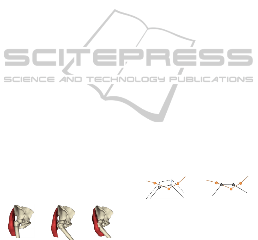
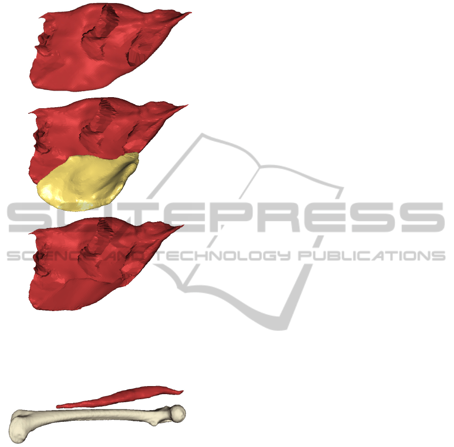
An example can be seen in Figure 1.

Figure 1: Position of bones (pelvis and femur) and shape

of the gluteus maximus: a) muscle and bones in RP;

b) bones in CP, muscle in RP; c) muscle deformed to CP.

The original method is based on algorithm de-

scribed in (Huang et al., 2006). For each muscle, its

outer hull (a low polygon coarse mesh) is needed.

Mostly it is loaded from the pre-computed database;

if not available, the hull is computed by the progres-

sive hull decimation algorithm (Cholt, 2012). This

coarse hull is used to get an initial approximate solu-

tion, which is then refined by a final few iterations in

which the original mesh is used. This strategy saves

both memory and computational power.

The deformation algorithm as described in

(Kellnhofer et al., 2012) defines constraints to pre-

serve the shape of the muscle, its main deformation

direction and its volume. From these constraints the

over-constrained linear system with non-linear

boundary constraint of volume was mathematically

derived. We solve the equations iteratively using

Gauss-Newton method with Lagrange coefficients.

In each iterative step, a new position for every ver-

tex of the mesh being processed (either the coarse

hull mesh or the full mesh) is computed, after which

the intersection corrections are applied to avoid

mutual inter-penetration of meshes.

3.1 Solving Intersections

During the whole deformation, computation inter-

sections are solved on two levels. In each iterative

step, it is checked, if the deformation has not moved

the mesh vertices too far. Because it profits from the

knowledge of the previous vertex position and its

motion, it is called dynamic intersection. As can be

seen in Figure 2, if any vertex is found to lie inside

an obstacle, the adequate triangle of the obstacle in

the direction inverse to the vertex motion direction is

detected and the vertex is moved to the boundary of

the obstacle (on the detected triangle) – left gray

point in Figure 2; or to its previous position, if the

vertex has been already inside the obstacle before

the deformation step – right gray point in Figure 2.

Figure 2: Dynamic intersection solving schema (colour

curve represents the obstacle, black curve the deforming

muscle): a) the original position of vertices (solid line) and

the intersected vertices after deformation iteration (dashed

line); b) situation after intersection solving.

As each vertex of the original muscle mesh is de-

fined as the linear combination of all vertices of the

hull, the linear mapping is not able to represent a

larger pit pushed into the original mesh surface and,

therefore, after all iterations, the final intersection

check, called static intersection, using full meshes

must be done to prevent problems.

GRAPP2013-InternationalConferenceonComputerGraphicsTheoryandApplications

Because we need to check the relative position of

muscles and obstacles, we cannot use any infor-

mation about the previous movement; the detection

starts from the relative positions of computed mesh-

es. Intersected vertices are grouped, for each group

its central point is computed (as an average position

of all group vertices) and all vertices of the group

are moved to the nearest triangle of the intersected

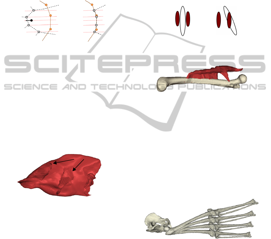
object. An example can be seen in Figure 3.

a) b)

Figure 3: Static intersection solving schema: a) central

point position and direction of vertices movement (red

dotted lines); b) intersected vertices moved to the correct

position on the border of the obstacle surface.

4 INTERPOLATION METHOD

The original deformation method described above

works well and quite quickly. But when we have a

look on its result in detail (e.g. in Figure 4) the sharp

cut of the bone into the muscle surface computed by

the original method can be seen well (in this exam-

ple pelvis bone and the gluteus maximus were used).

The enlarged detail can be also found in Figure 12a.

Figure 4: Result of the original deformation method.

This result is caused by static intersection being

solved just once. It would be advantageous to run

the static intersection solving several times to keep

the print of bones in muscles smooth and to deform

muscles more realistically.

Another problem emerges, if we have two muscles

touching a bone in RP, as it is outlined in Figure

5(a). After moving the bone into CP, the bone inter-

sects one of these muscles completely (b). As the

dynamic intersections are being solved in each itera-

tion step, the muscle vertices, which are intersected

before the deformation, remain intersected. The

result can be seen in Figure 6: the shape of the mus-

cle is incorrect as the muscle is fixed on the bone.

The basic idea of the proposed modification is sim-

ple: if the distance between RP and CP positions is

too large, we create several artificial inter-steps in

between because the static intersection will then

move the muscle mesh vertices for a smaller dis-

tance and one can expect that sharp unrealistic-

looking pits would be avoided. To create these inter-

steps, we have to interpolate all obstacles and also

action lines. Both interpolations are described in the

following sections.

a) b)

Figure 5: Schema of position of muscles and bone: a) all

in RP without any intersections; b) muscles before the

deformation in RP, bone already in CP.

Figure 6: Rectus femoris computed by the original defor-

mation method.

4.1 Bones Interpolation

As bones are represented by triangular meshes, their

vertices can be interpolated separately as:

=rp

+j*(cp

-rp

)/stepCoun

(1)

where x

are coordinates of the i-th vertex in the j-th

interpolation, rp

is the i-th vertex of the RP mesh,

represents coordinates of the same vertex in the

CP, stepCount determines the number of interpola-

tion steps. In Figure 7, all interpolation positions of

the right leg can be seen.

Figure 7: Pelvis, right thigh and shank bones in interpolat-

ed positions.

4.2 Action Lines Interpolation

As the poly-lines representing the RP and the CP

paths of the action line may not have the same num-

ber of points, or the distribution of points along

these poly-lines may be very different, first we must

ensure that both poly-lines are matched (both have

MusculoskeletalSystemModelling-InterpolationMethodforMuscleDeformation

the same number and distribution of points) to simp-

ly interpolate them.

Let us assume that the RP poly-line C is formed

by the points P

... P

and the CP poly-line C' by the

points P

' ... P

'. The matching starts with an

arc-length parameterization of both poly-lines, i.e.,

to points P

and P

', we assign the parameters t

and

', respectively, such that:

























´´

(2)

Hence t

= t´

= 0 and t

= t´

= 1.

The points of the RP poly-line are now pro-

cessed. Given the point P

, the algorithm searches, in

increasing values of j, for a point P

 that has not

been already matched and for which |t

- t

'| is small-

er than some allowed tolerance ε. If the outcome of

the search is negative, a new point P

' is introduced

on the CP poly-line at the location for which the

parameter value t

' = t

. The points P

and P

' are then

said to be matched. Any as-yet-unmatched points on

the CP poly-line are then processed using a similar

approach. By the end of this process, both poly-lines

will have the same number of points and these points

will be matched. The overall matching process is

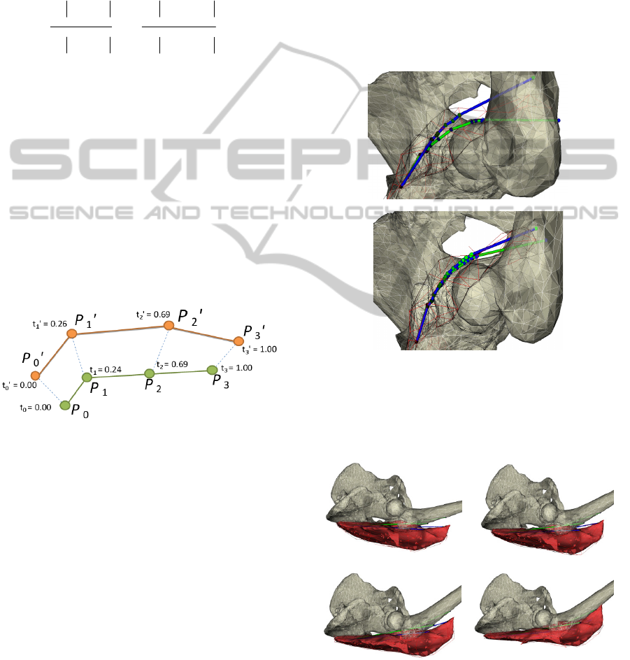
shown in Figure 8.

Figure 8: Matching the RP poly-line P

, P

and the CP

poly-line P

’, P

’ – arc-length parameterization of

both poly-lines.

When RP and CP action lines are matched, the

interpolation can be done in the same manner as in

the case of bones. In Figure 9a, the original action

lines and their points can be seen (action line in RP

is represented by the green curve with blue points,

the action line in CP is figured as blue curve with

green points). Figure 9b shows the matched RP

action line and the interpolated first step action line.

The triangle mesh around the action lines is the hull

of deformed muscle hull in RP.

4.3 Deformation Computation

Let us assume three-step interpolation (the number

of steps can be specified either by the user or com-

puted automatically from the largest distance differ-

ence between the vertices of the original RP and

CP), i.e., we have four positions: RP = P

(see Fig-

ure 10a), P

, P

and P

= CP. The method starts with

the calculation of paths of action lines and positions

of vertices of bones at P

and P

using linear interpo-

lation of those at P

and P

. Afterwards, the original

deformation method is run to wrap muscles from P

into P

(Figure 10b), after which it is run again to

wrap muscles from P

to P

(Figure 10c) and finally,

in a successive run, to wrap these muscles into the

final position P

(Figure 10d).

Figure 9: Action lines of illiacus; RP (the more curved

one) is surrounded by the triangle surface of muscle hull:

a) the original action lines (green curve with blue points in

RP, blue curve with green points in CP); b) recomputed

action lines for the first step of the interpolation.

c) d)

Figure 10: Steps of the interpolation process: a) RP of the

muscle and first interpolated position of bones and action

lines (P

); b, c) starting position of second and third inter-

polation steps (P

and P

); d) final deformation state of the

muscle (P

GRAPP2013-InternationalConferenceonComputerGraphicsTheoryandApplications

5 RESULTS

Figure 11 shows the impact of the proposed new

method on the static intersection in the case of glu-

teus maximus and pelvis. The original method (a)

shifts the vertices for approx. double distances than

the interpolation method (b) and majority of them

are shifted for a similar distance, while in the new

method the shifting distance decreases to the borders

of the intersected area. This means that the created

bone print shape is smoother. Moreover, each fol-

lowing interpolation step deforms the semi-result

and so any sharp edge is smoothed.

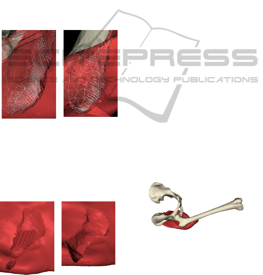
a) b)

Figure 11: Static intersection solving (line segments repre-

sent the trajectory of moved vertices): a) at the end of the

original method computation; b) during the last interpola-

tion step.

Figure 12 compares the shapes of muscles de-

formed by both methods. It can be seen that the

muscle provided by the new method does not con-

tain any sharp edges of the pit and the gradual bor-

ders of the pit seems to correspond more with the

real forming of a consistent muscle.

a) b)

Figure 12: Result of contact area of gluteus maximus and

pelvis computed by: a) the original method; b) the interpo-

lated deformation method.

The only problem, which has yet to be resolved, is

the high computational time. Its main reason is that

it is necessary to construct a new hull before each

step because the static intersection solving at the end

of the interpolation step modifies the original mesh

and while it is possible to easily get the original

mesh from the hull (thanks to the linear mapping of

vertices) it is not possible so far to provide the re-

verse process. The computation of muscle defor-

mation needs just several seconds to get results, as

mentioned already in (Kellnhofer et al., 2012). If we

provide it several times to get the interpolation semi-

results, the computation needs still seconds to finish,

but before each interpolation step the outer low

polygon hull has to be computed again.

The progressive hulls decimation algorithm

needs easily a minute on commodity hardware to

compute a new hull and if we need to repeat it sev-

eral times during the whole interpolation, the com-

putational time grows with each single step. Because

it is not possible to provide the whole computation

on a hull or to avoid the static intersections, our

future research will be focused on possible ap-

proaches on reverse (full mesh to hull) computation.

So far one single muscle deformation together

with surrounding bones was described. The human

body contains of course many muscles which are

placed close to each other and so if more muscles

are taken into the deformation method, it should

keep the bilateral influence. Figure 14a shows the

difference between the single muscle deformation.

The muscle together with involved bones can be

seen also in Figure 13. Parallel deformation of glu-

teus maximus and gluteus medius is shown in Figure

14b-c. (in Figure 14c, only gluteus maximus is visu-

alized and so impact of gluteus medius is visible in

the bottom part of the visualized muscle).

Figure 13: Gluteus maximus computation; computed

bones (pelvis and femur) are visualized.

There was one more problem described in Sec-

tion 4: fixing of the muscle on the bone because of

the dynamic intersections. The result of interpolation

method for the used example – rectus femoris can be

seen in Figure 15. Thanks to the smaller movements

of the bone, no problems appeared.

MusculoskeletalSystemModelling-InterpolationMethodforMuscleDeformation

Figure 14: Results of the interpolated deformation method

(4 steps of interpolation were used): a) gluteus maximus

computed only with bones (no other muscle); b) gluteus

maximus computed together with gluteus medius; c) visu-

alization of result from (b), gluteus medius is hiden.

Figure 15: Rectus femoris computed by the interpolated

deformation method.

6 CONCLUSIONS

We have developed method for deformation of mus-

cles in the musculoskeletal model of human body.

Despite of its high computational time (though it is

still much lower than in case of FEM methods), the

interpolation method seems to be an interesting

supplement to the currently used one-pass defor-

mation method especially in such parts of the model,

where the difference between the initial and final

position of bones is too large to provide the compu-

tation at once and where the large bones are pressed

into muscles. Moreover, the further research and

optimization of original mesh to muscle hull conver-

sion may help to decrease the computational time so

that the well looking results could be used also in the

real time model processing.

ACKNOWLEDGEMENTS

This work was partly supported by the Information

Society Technologies Programme of the European

Commission under the project VPHOP (FP7-ICT-

223865).

The authors would like to thank the various peo-

ple who provided condition under which the work

could be done.

REFERENCES

AnyBody technology (2010), available from

http://www.anybodytech.com

Blanco F. R., Oliveira M. M. (2008), Instant mesh defor-

mation, In: Proceedings of the 2008 Symposium on In-

teractive 3D Graphics and Games, Redwood City,

California, 71-78.

Blemker S. S., Delp S. L. (2005), Three-dimensional

representation of complex muscle architectures and

geometries, Annals of Biomedical Engineering 33,

661-673.

Cholt D. (2012), Progressive hulls: application on biomed-

ical data, In Proceedings of the 16th Central European

Seminar on Computer Graphics CESCG 2012, Slo-

vakia, 9-16, ISBN 978-3-9502533-4-4.

Huang, J., Shi, X., Liu, X., Zhou, K., Wei, L.Y., Teng, S.

H., Bao, H., Guo, B., and Shum, H. Y. (2006). Sub-

space gradient domain mesh deformation. ACM

Transactions on Graphics, 25(3): 1126–1134.

Ju T., Schaefer S., Warren J. (2005), Mean value coordi-

nates for closed triangular meshes, ACM Transactions

on Graphics 24 (3): 561–566.

Kellnhofer P., Kohout J. (2012), Time-Convenient Defor-

mation of Musculoskeletal System, In Proceedings of

Conference on Scientific Computing Algoritmy 2012,

Slovakia.

OpenSim project (2010), available from

https://simtk.org/home/opensim.

Richardson M. (2001), Muscle Atlas of the Extremities,

Amazon Whispernet.

Shi, X., Zhou K., Tong Y., Desbrun M., Bao H., Guo B.

(2007) Mesh Puppetry: Cascading Optimization of

Mesh Deformation with Inverse Kinematics, ACM

Transactions on Graphics - Proceedings of ACM

SIGGRAPH 2007, 26(3), ACM New York.

VPHOP (2012). the osteoporotic virtual physiological

human, http://vphop.eu/.

GRAPP2013-InternationalConferenceonComputerGraphicsTheoryandApplications