Emergent Segmentation of Topological Active Nets by Means of

Evolutionary Obtained Artiﬁcial Neural Networks

Cristina V. Sierra, Jorge Novo, Jos

e Santos and Manuel G. Penedo

Computer Science Department, University of A Coru

na, A Coru

na, Spain

Keywords:

Image Segmentation, Topological Active Nets, Differential Evolution, Artiﬁcial Neural Networks.

Abstract:

We developed a novel segmentation method using deformable models. As deformable model we used Topo-

logical Active Nets, model which integrates features of region-based and boundary-based segmentation tech-

niques. The deformation through time is deﬁned by an Artiﬁcial Neural Network (ANN) that learns to move

each node of the segmentation model based on its energy surrounding. The ANN is applied to each of the

nodes and in different temporal steps until the ﬁnal segmentation is obtained. The ANN training is obtained

by simulated evolution, using differential evolution to automatically obtain the ANN that provides the emer-

gent segmentation. The new proposal was tested in different artiﬁcial and real images, showing the capabilities

of the methodology.

1 INTRODUCTION AND

PREVIOUS WORK

The active nets model for image segmentation was

proposed (Tsumiyama and Yamamoto, 1989) as

a variant of the deformable models (Kass et al.,

1988) that integrates features of region–based and

boundary–based segmentation techniques. To this

end, active nets distinguish two kinds of nodes: in-

ternal nodes, related to the region–based information,

and external nodes, related to the boundary–based in-

formation. The former model the inner topology of

the objects whereas the latter ﬁt the edges of the ob-

jects. The Topological Active Net (TAN) (Ansia et al.,

1999) model was developed as an extension of the

original active net model. It solves some intrinsic

problems to the deformable models such as the initial-

ization problem. It also has a dynamic behavior that

allows topological local changes in order to perform

accurate adjustments and ﬁnd all the objects of inter-

est in the scene. The model deformation is controlled

by energy functions in such a way that the mesh en-

ergy has a minimum when the model is over the ob-

jects of the scene. This way, the segmentation process

turns into a minimization task.

The energy minimization of a given deformable

model has been faced with different minimization

techniques. One of the simplest methods is the greedy

strategy (Williams and Shah, 1992). The main idea

implies the local modiﬁcation of the model in a way

the energy of the model is progressively reduced. The

segmentation ﬁnishes when no further modiﬁcation

implies a reduction in terms of energy. As the main

advantages, this method is fast and direct, providing

the ﬁnal segmentations with low computation require-

ments. However, as a local minimization method, it

is also sensitive to possible noise or complications in

the images. This method was used as a ﬁrst approxi-

mation to the energy minimization of the Topological

Active Nets (Ansia et al., 1999).

As the local greedy strategy presented relevant

drawbacks, especially regarding the segmentation

with complex and noisy images, different global

search methods based on evolutionary computation

were proposed. Thus, a global search method using

genetic algorithms (Ib

nez et al., 2009) was designed.

As a global search technique, this method provided

better results working under different complications

in the image, like noise or fuzzy and complex bound-

aries, situations quite common working under real

conditions. However, this approach presented an im-

portant drawback, that is the complexity. The seg-

mentation process needed large times and computa-

tion requirements to reach the desired results. As an

improvement of the genetic algorithm approach, an-

other evolutionary optimization technique was pro-

posed (Novo et al., 2011). This new approach, based

in differential evolution, allowed a simpliﬁcation of

the previous method and also speed up the segmenta-

tion process, obtaining the ﬁnal results in less genera-

V. Sierra C., Novo J., Santos J. and G. Penedo M..

Emergent Segmentation of Topological Active Nets by Means of Evolutionary Obtained Artiﬁcial Neural Networks.

DOI: 10.5220/0004195700440050

In Proceedings of the 5th International Conference on Agents and Artiﬁcial Intelligence (ICAART-2013), pages 44-50

ISBN: 978-989-8565-39-6

 2013 SCITEPRESS (Science and Technology Publications, Lda.)

tions (implying less time).

There is very little work regarding emerging sys-

tems and deformable models for image segmenta-

tion. “Deformable organisms” were used for an au-

tomatic segmentation in medical images (McInerney

et al., 2002). Their artiﬁcial organisms possessed de-

formable bodies with distributed sensors, while their

behaviors consisted of movements and alterations of

predeﬁned body shapes (deﬁned in accordance with

the image object to segment). The authors demon-

strated the method with several prototype deformable

organisms based on a multiscale axisymmetric body

morphology, including a “corpus callosum worm” to

segment and label the corpus callosum in 2D mid-

sagittal MR brain images.

In this paper, we used Differential Evolution (DE)

(Price and Storn, 1997)(Price et al., 2005) to train

an Artiﬁcial Neural Network (ANN) that works as

a “segmentation operator” that knows how to move

each TAN node in order to reach the ﬁnal segmenta-

tions. Section 2 details the main characteristics of the

method. It includes the basis of the Topological Ac-

tive Nets, deformable model used to achieve the seg-

mentations (Sub-section 2.1), the details of the ANN

designed (Sub-section 2.2) and the optimization of the

ANN parameters using the DE method (Sub-section

2.3). In Section 3 different artiﬁcial and real images

are used to show the results and capabilities of the ap-

proach. Finally, Section 4 expounds the conclusions

of the work.

2 METHODS

2.1 Topological Active Nets

A Topological Active Net (TAN) is a discrete imple-

mentation of an elastic n−dimensional mesh with in-

terrelated nodes (Ansia et al., 1999). The model has

two kinds of nodes: internal and external. Each kind

of node represents different features of the objects:

the external nodes ﬁt their edges whereas the internal

nodes model their internal topology.

As other deformable models, its state is governed

by an energy function, with the distinction between

the internal and external energy. The internal en-

ergy controls the shape and the structure of the net

whereas the external energy represents the external

forces which govern the adjustment process. These

energies are composed of several terms and in all the

cases the aim is their minimization.

Internal Energy Terms. The internal energy de-

pends on ﬁrst and second order derivatives which con-

trol contraction and bending, respectively. The inter-

nal energy term is deﬁned through the following equa-

tion for each node:

int

(v(r, s)) = α (|v

(r, s)|

+ |v

(r, s)|

) +

β (|v

(r, s)|

+ |v

(r, s)|

+ |v

(r, s)|

)

(1)

where the subscripts represent partial derivatives, and

α and β are coefﬁcients that control the ﬁrst and sec-

ond order smoothness of the net. The ﬁrst and second

derivatives are estimated using the ﬁnite differences

technique.

External Energy Terms. The external energy repre-

sents the features of the scene that guide the adjust-

ment process:

ext

(v(r, s)) = ω f [I(v(r,s))]+

|ℵ(r, s)|

∑

p∈ℵ(r,s)

||v(r,s)−v(p)||

f [I(v(p))]

(2)

where ω and ρ are weights, I(v(r,s)) is the intensity of

the original image in the position v(r,s), ℵ(r,s) is the

neighborhood of the node (r,s) and f is a function,

which is different for both types of nodes since the

external nodes must ﬁt the edges whereas the internal

nodes model the inner features of the objects.

If the objects to detect are bright and the back-

ground is dark, the energy of an internal node will

be minimum when it is on a point with a high grey

level. Also, the energy of an external node will be

minimum when it is on a discontinuity and on a dark

point outside the object. Given these circumstances,

the function f is deﬁned as:

f [I(v(r, s))] =











(v(r, s)) + τIOD

(v(r, s)) for internal nodes

(v(r, s)) + τIOD

(v(r, s)) + for external

ξ(G

max

− G(v(r, s))) + δGD(v(r,s)) nodes

(3)

where τ, ξ and δ are weighting terms, G

max

and

G(v(r, s)) are the maximum gradient and the gradient

of the input image in node position v(r,s), I(v(r,s))

is the intensity of the input image in node position

v(r, s), IO is a term called “In-Out” and IOD a term

called “distance In-Out”, and GD(v(r,s)) is a gradi-

ent distance term. The IO term minimizes the energy

of individuals with the external nodes in background

intensity values and the internal nodes in object inten-

sity values meanwhile the terms IOD act as a gradi-

ent: for the internal nodes (IOD

) its value minimizes

towards brighter values of the image, whereas for the

external nodes its value (IOD

) is minimized towards

low values (background).

The adjustment process consists of minimizing

these energy functions, considering a global energy as

the sum of the different energy terms, weighted with

the different exposed parameters, as used in the opti-

mizations with a greedy algorithm (Ansia et al., 1999)

or with an evolutionary approach (Ib

nez et al., 2009;

Novo et al., 2011).

EmergentSegmentationofTopologicalActiveNetsbyMeansofEvolutionaryObtainedArtificialNeuralNetworks

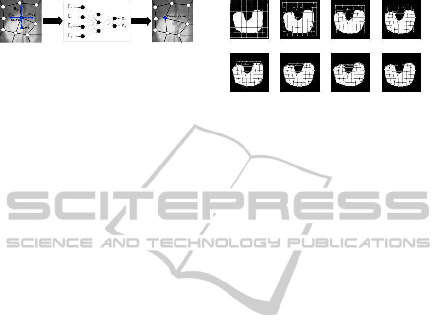
Figure 1: Diagram of the shift production for a given TAN

node using the ANN.

2.2 Artiﬁcial Neural Networks for the

Image Segmentation

A new segmentation technique that uses Artiﬁcial

Neural Networks (ANNs) to perform the optimiza-

tion of the Topological Active Nets is proposed in this

work. In particular, we used a classical multilayer per-

ceptron model that is trained to know how the TAN

nodes have to be moved and reach the desired seg-

mentations.

The main purpose of the ANNs consist of pro-

viding, for a given TAN node, the most suitable

movement that implies an energy minimization of the

whole TAN structure. This is not the same as the

greedy algorithm, which determines the minimization

for each node movement. All the characteristics of the

network were designed to obtain this behavior, and

are the following:

Input. The ANN is applied iteratively to each of the

TAN nodes. The network has as input the four hy-

pothetical energy values that would take the mesh

if the given node was moved in the four cardinal

directions. Moreover, these values are normalized

with respect to the energy in the present position,

given the high values that the energy normally

takes, following the formula:

= (E

− E

)/E

(4)

where E

is the given hypothetical energy to be

normalized and E

is the energy with the TAN

node in the present location.

Hidden Layers. One single hidden layer composed

by a different number of nodes. The sigmoid

transfer function was used for all the nodes.

Output. The network provides the movement that

has to be done in each axis for the given TAN

node. So, it has two output nodes that specify the

shift in both directions of the current position.

These characteristics can be seen in Figure 1. In

this case, we obtain the values of the hypothetical en-

ergies that would be taken if we move the central node

in the x and y axes, represented by the E

x−

y−

and E

values. These are introduced as the input val-

ues in the corresponding ANN, that produces, in this

example, a horizontal displacement for the given TAN

Step 0 Step 9 Step 23 Step 31

Step 38 Step 47 Step 52 Step 65

Figure 2: Emergent segmentation provided by the ANN in

different steps.

node. This movement, provided by the network out-

puts, is restricted in a small interval of pixels around

the current position, typically between 1 and 5 pixels

in both axes and directions.

Once we have the ANN correctly trained (with the

evolutionary algorithm), we can use it as a “segmenta-

tion operator” that progressively moves the entire set

of TAN nodes until, after a given number of steps, the

TAN reaches the desired segmentation. In this pro-

cess, the ANN is applied to each of the nodes sequen-

tially. Such a temporal “step” is the application of

the ANN to all the nodes of the TAN. An example of

segmentation is shown in Figure 2, where the TAN

was established initially in the limits of the image and

all the nodes were moved until a correct segmentation

was reached.

2.3 Differential Evolution for the

Optimization of the Artiﬁcial

Neural Network

Differential Evolution (DE) (Price and Storn,

1997)(Price et al., 2005) is a population-based

search method. DE creates new candidate solutions

by combining existing ones according to a simple

formula of vector crossover and mutation, and then

keeping whichever candidate solution which has the

best score or ﬁtness on the optimization problem at

hand. The central idea of the algorithm is the use

of difference vectors for generating perturbations in

a population of vectors. This algorithm is specially

suited for optimization problems where possible so-

lutions are deﬁned by a real-valued vector. The basic

DE algorithm is summarized in the pseudo-code of

Figure 3.

One of the reasons why Differential Evolution is

an interesting method in many optimization or search

problems is the reduced number of parameters that

are needed to deﬁne its implementation. The parame-

ters are F or differential weight and CR or crossover

probability. The weight factor F (usually in [0, 2])

ICAART2013-InternationalConferenceonAgentsandArtificialIntelligence

1. Initialize all individuals x with random

positions in the search space

2. Until a termination criterion is met,

repeat the following:

For each individual x in the population do:

2.1 Pick three random individuals x

from the population they must be distinct

from each other and from individual x.

2.2 Pick a random index Rε1,...,n, where the

highest possible value n is the dimensionality

of the problem to be optimized.

2.3 Compute the individual’s potentially new position

y = [y

,...,y

] by iterating over each iε1,...,n as follows:

2.3.1 Pick r

εU (0, 1) uniformly from the open

range (0,1).

2.3.2 If (i = R) or (r

< CR)

let y

= x

+ F (x

− x

), otherwise let y

= x

2.4 If ( f (y) < f (x)) then replace the individual x

in the population with the improved candidate

solution, that is, set x = y in the population.

3. Pick the individual from the population that has the

lowest fitness and return it as the best found

candidate solution.

Figure 3: Differential Evolution Algorithm.

is applied over the vector resulting from the differ-

ence between pairs of vectors (x

and x

). CR is the

probability of crossing over a given vector (individ-

ual) of the population (x

) and a vector created from

the weighted difference of two vectors (F(x

− x

)),

to generate the candidate solution or individual’s po-

tentially new position y. Finally, the index R guaran-

tees that at least one of the parameters (genes) will be

changed in such generation of the candidate solution.

One of the main advantages of DE is that it pro-

vides an automatic balance in the search. As it was

indicated (Feoktistov, 2006), the fundamental idea of

the algorithm is to adapt the step length (F(x

− x

))

intrinsically along the evolutionary process. At the

beginning of generations the step length is large, be-

cause individuals are far away from each other. As

the evolution goes on, the population converges and

the step length becomes smaller and smaller.

2.3.1 ANN Genotypic Encoding

In our application, a single ANN was used to learn

the movements that have to be done by the internal

and the external nodes. In the evolutionary popula-

tion, each individual encodes the ANN. The geno-

types code all the weights of the connections between

the different nodes of the ANN. The weights were en-

coded in the genotypes in the range [−1,1], and de-

coded to be restricted in an interval [-MAX VALUE,

MAX VALUE]. In the current ANN used, the inter-

val [−1,1] was enough to determine output values in

the whole range of the transfer functions of the nodes.

We initialized the TAN nodes in the borders of the

images and applied a ﬁxed number of steps. Each step

consists of the modiﬁcation produced by the ANN for

each of the nodes of the TAN. Finally, the ﬁtness as-

sociated to each individual or encoded ANN is the en-

ergy that has the ﬁnal conﬁguration of the TAN which

must be minimized. So, the ﬁtness is deﬁned only by

the ﬁnal emergent segmentation provided by an en-

coded ANN.

Moreover, the usual implementation of DE

chooses the base vector x

randomly or as the indi-

vidual with the best ﬁtness found up to the moment

best

). To avoid the high selective pressure of the

latter, the usual strategy is to interchange the two pos-

sibilities across generations. Instead of this, we used

a tournament to pick the vector x

, which allows us to

easily establish the selective pressure by means of the

tournament size.

3 RESULTS

Different representative artiﬁcial and real CT images

were selected to show the capabilities and advantages

of the proposed method. Regarding the evolutionary

DE optimization, all the processes used a population

of 1000 individuals and the tournament size to select

the base individual x

in the DE runs was 5% of the

population. We used a ﬁxed value for the CR param-

eter (0.9) and for the F parameter (0.9). These values

provided the best results in all the images. In the cal-

culation of the ﬁtness of the individual, we applied a

number of steps between 50 and 400, depending on

the complexity and the resolution of the image.

Table 1 includes the energy TAN parameters used

in the segmentation examples. Those were experi-

mentally set as the ones in which the corresponding

ANN gave the best results for each training.

Table 1: TAN parameter sets used in the segmentation pro-

cesses of the examples.

Figures Size α β ω ρ ξ δ τ

4,5,6 8 × 8 1.0 1.0 10.0 4.0 0.0 6.0 30.0

7 12 × 12 0.0 2.0 20.0 3.0 0.0 5.0 0.0

9 8 × 8 4.5 0.8 10.0 2.0 7.0 20.0 40.0

10 8 × 8 4.5 0.8 10.0 2.0 7.0 20.0 40.0

3.1 Segmentation of Artiﬁcial Images

Firstly, we tested the methodology with artiﬁcial im-

ages with different characteristics. In this case, we

used a training set of 4 artiﬁcial images, each one with

different characteristics (different shapes, inclusion of

EmergentSegmentationofTopologicalActiveNetsbyMeansofEvolutionaryObtainedArtificialNeuralNetworks

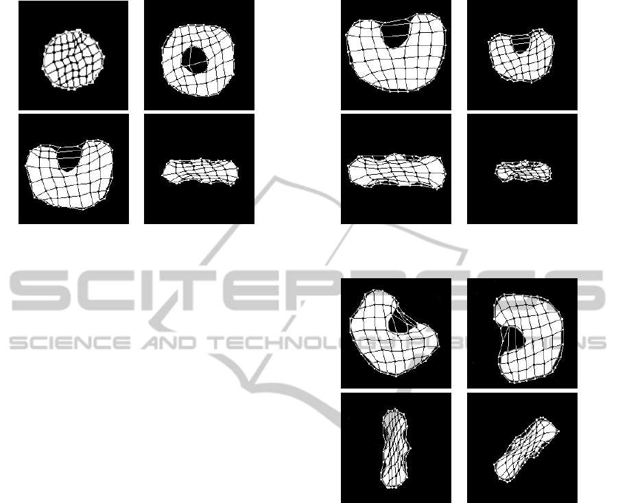
Figure 4: Results obtained with the best ANN for the seg-

mentation of the training images.

concavities, holes, etc.). The ﬁtness is deﬁned as the

sum of the individual ﬁtnesses provided by the same

ANN (individual) in all the training images.

Figure 4 shows the ﬁnal segmentations obtained

with the training set. Moreover, we tested the trained

ANNs with a different set of images. Once we have

the ANNs trained, the segmentation is fast and direct,

applying the modiﬁcations to the TAN nodes a given

number of steps until we reach the ﬁnal segmentation.

Note that two of the images have great difﬁculties for

a perfect segmentation, with a big hole and a deep

concavity, so some nodes can incorrectly fall in the

hole or the concavity. For testing the trained ANN,

we scaled and rotated a couple of difﬁcult images of

the training dataset, to verify the independence of the

training regarding modiﬁcations in the used objects.

Figures 5 and 6 show the ﬁnal results with the test

set of images. As the Figures show, the ANNs are

able to reach correct results, which demonstrates that

the ANN has learned to move correctly the nodes, in-

dependently of the training image or images used, to

provide a ﬁnal correct segmentation.

3.2 Comparison of the proposed

Method and the Greedy Algorithm

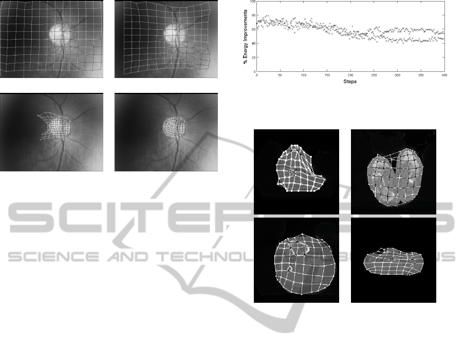
We compared the proposed method with respect to the

greedy approach previously deﬁned. We selected a

domain with real difﬁcult images, as we segmented

the optic disc in eye fundus images, as detailed in

(Novo et al., 2009). The objective is the segmentation

of the optic disc (oval bright area in the image) which

also provides the localization of the center of the op-

tic disc. As Figure 7 shows, the greedy local search

falls in local minima quite fast, being impossible to

reach the optic disc boundary (Figure 7 (a)). On the

Figure 5: Results obtained when the best ANN is tested

with scaled artiﬁcial objects.

Figure 6: Results obtained when the best ANN is tested

with rotated artiﬁcial objects.

contrary, the ANN learned how to move all the nodes

and was capable to reach an acceptable result (Figure

7 (b)–(d)). Note the capability of the evolved ANN

to overcome the high level of noise, that prevents the

correct segmentations by the greedy methodology.

In this case, additionally to the TAN energy pa-

rameters depicted in Table 1, we also used the ad-hoc

energy terms designed for this speciﬁc task, as de-

tailed in (Novo et al., 2009). These energy terms are

“circularity”, that potentiates a circular shape of the

TAN, and “contrast of intensities”, that tries to put

the external nodes in locations with bright intensities

in the inside and dark intensities outside. This term

was designed to avoid the falling of the external nodes

in the inner blood vessels. In this segmentation, the

corresponding energy parameters of these two ad-hoc

energy terms took values of cs = 30.0 and ci = 15.0,

respectively.

To explain why the greedy local search and the

ICAART2013-InternationalConferenceonAgentsandArtificialIntelligence

(a) (b)

Figure 7: Comparison between the greedy algorithm and

the proposed method. (a) Final result with the greedy ap-

proach. (b)–(d) Segmentation provided by the ANN in dif-

ferent temporal steps: 30, 171 and 399.

proposed method behave differently, we included, in

Figure 8, a graphic with the percentage of the TAN

node shifts that implied a maintenance or improve-

ment (decrement) in terms of energy, and for each

step in the segmentation of the optic disc of Figure

7. In the graphic, the main difference between the

proposed method and the greedy local search is clear.

Using the greedy method, all the movements of the

TAN nodes imply a new position with an energy at

least the same as the previous one, and better if pos-

sible (100% in the graph). That is why, in this par-

ticular segmentation, the greedy method falls in local

minima, because the nodes cannot ﬁnd a better posi-

tion in the neighborhood and in few steps. However,

with the proposed method, the ANN learned to pro-

duce “bad” movements (an average of 50% at the ﬁnal

steps), that implied worse energies in the short term,

but they were suitable to ﬁnd a correct segmentation

in terms of the entire segmentation process.

3.3 Segmentation of Real Images

Moreover, as in the case with artiﬁcial images, we

trained the ANNs with a given set of medical CT im-

ages, and after that, we tested the method with a dif-

ferent dataset. We selected a set of images that in-

cluded objects with different shapes and with differ-

ent levels of complexity. The CT images correspond

to a CT image of the head, the feet, the knee and a

CT image at the level of the shoulders. The images

used in the testing correspond to CT images of the

same close areas, but with a slightly different shape

and with deeper concavities. All these CT images pre-

sented some noise surrounding the object, noise that

Figure 8: Percentage of TAN node movements with an en-

ergy maintenance or improvement, over the temporal steps,

and using the trained ANN in the segmentation of Figure 7.

Figure 9: Results obtained with the best evolved ANN and

the training set of real CT images.

was introduced by the capture machines when obtain-

ing the medical CT images.

Figure 9 includes the ﬁnal segmentations with the

training dataset, whereas Figure 10 details the ﬁnal

segmentations obtained with the best trained ANN

and the test set of images. In both cases, the evolved

ANN was capable to provide acceptable results, in-

cluding a correct boundary detection and overcoming

the presence of noise in the images.

Again, in the difﬁcult parts of the images, like the

concavities, some external nodes fall incorrectly in

the background. This can be improved changing the

energy parameters, increasing the TAN energy GD

(Gradient Distance), but it deteriorates other objec-

tives like smoothness. So, the energy parameters are

always a compromise to obtain acceptable results in

different kind of images.

4 CONCLUSIONS

We proposed a new methodology for image segmen-

tation using deformable models. We used Topological

Active Nets as extended model which integrates fea-

tures of region-based and boundary-based segmenta-

EmergentSegmentationofTopologicalActiveNetsbyMeansofEvolutionaryObtainedArtificialNeuralNetworks

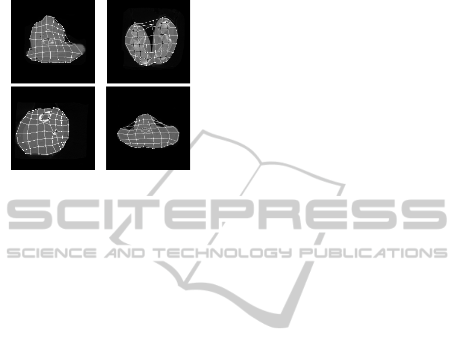
Figure 10: Results obtained with the best evolved ANN and

the test dataset of real CT images.

tion techniques. The deformation through time was

deﬁned by an evolutionary trained ANN, since the

ANN determined the movements of each one of the

nodes. The process was repeated for all the nodes and

in different temporal steps until the ﬁnal segmentation

was obtained.

Thus, the ANN provides an “emergent” segmen-

tation, as a result of the local movements provided by

the ANN and the local and surrounding energy infor-

mation that the ANN receives as input. The methodol-

ogy was proved successful in the segmentation of dif-

ferent artiﬁcial and real images, and overcoming noise

problems. Moreover, we tested the ANN, trained with

a set of images, with different testing images, obtain-

ing acceptable results. So, our trained ANNs can be

considered as “segmentation operators”.

ACKNOWLEDGEMENTS

This paper has been partly funded by the Ministry

of Science and Innovation through grant contracts

TIN2011-25476 and TIN2011-27294 and by the Con-

seller

ıa de Industria, Xunta de Galicia through grant

contract 10/CSA918054PR using FEDER funds.

REFERENCES

Ansia, F., Penedo, M., Mari

no, C., and Mosquera, A.

(1999). A new approach to active nets. Pattern Recog-

nition and Image Analysis, 2:76–77.

Feoktistov, V. (2006). Differential Evolution: In Search of

Solutions. Springer, New York, USA.

nez, O., Barreira, N., Santos, J., and Penedo, M. (2009).

Genetic approaches for topological active nets opti-

mization. Pattern Recognition, 42:907–917.

Kass, M., Witkin, A., and Terzopoulos, D. (1988). Snakes:

Active contour models. International Journal of Com-

puter Vision, 1(2):321–323.

McInerney, T., Hamarneh, G., Shenton, M., and Terzopou-

los, D. (2002). Deformable organisms for automatic

medical image analysis. Medical Image Analysis,

6:251–266.

Novo, J., Penedo, M. G., and Santos, J. (2009). Locali-

sation of the optic disc by means of GA-Optimised

Topological Active Nets. Image and Vision Comput-

ing, 27:1572–1584.

Novo, J., Santos, J., and Penedo, M. G. (2011). Optimiza-

tion of Topological Active Nets with differential evo-

lution. Lecture Notes in Computer Science: Adaptive

and Natural Computing Algorithms, 6593:350–360.

Price, K. and Storn, R. (1997). Differential evolution - a

simple and efﬁcient heuristic for global optimization

over continuous spaces. Journal of Global Optimiza-

tion, 11(4):341–359.

Price, K., Storn, R., and Lampinen, J. (2005). Differential

Evolution. A Practical Approach to Global Optimiza-

tion. Springer - Natural Computing Series.

Tsumiyama, K. and Yamamoto, K. (1989). Active net: Ac-

tive net model for region extraction. IPSJ SIG notes,

89(96):1–8.

Williams, D. J. and Shah, M. (1992). A Fast algorithm for

active contours and curvature estimation. CVGIP: Im-

age Understanding, 55(1):14–26.

ICAART2013-InternationalConferenceonAgentsandArtificialIntelligence