Wavelet-based Semblance for P300 Single-trial Detection

Carolina Saavedra

1,2

and Laurent Bougrain

1,2

Universit´e de Lorraine, LORIA, UMR 7503, Vandoeuvre-l`es-Nancy, F-54506, France

Inria, Villers-l`es-Nancy, F-54600, France

Keywords:

Event-related Potential, Denoising, Wavelets, Signals Correlation, Single-trial Detection, Brain-computer

Interfaces.

Abstract:

Electroencephalographic signals are usually contaminated by noise and artifacts making difﬁcult to detect

Event-Related Potential (ERP), specially in single trials. Wavelet denoising has been successfully applied to

ERP detection, but usually works using channels information independently. This paper presents a new adap-

tive approach to denoise signals taking into account channels correlation in the wavelet domain. Moreover, we

combine phase and amplitude information in the wavelet domain to automatically select a temporal window

which increases class separability. Results on a classic Brain-Computer Interface application to spell charac-

ters using P300 detection show that our algorithm has a better accuracy with respect to the VisuShrink wavelet

technique and XDAWN algorithm among 22 healthy subjects, and a better regularity than XDAWN.

1 INTRODUCTION

The analysis of brain activity with appropriate tech-

niques allows to extract properties of underlying neu-

ral activity and to better understand high level func-

tions. Wavelet are efﬁcient to process non-stationary

signals and can be useful to detect event-related po-

tentials (ERP) as the ones used in brain-computer in-

terface (BCI) systems.

A Brain-Computer Interface enables users to act

on either a real or a virtual environment by transcrib-

ing brain activity into commands for a computer ap-

plication or other devices (Wolpaw et al., 2002).

The P300 speller (Farwell and Donchin, 1988) is

a well-known BCI system which allows the user to

write text. It records the brain activity using an elec-

troencephalographic (EEG) system with several elec-

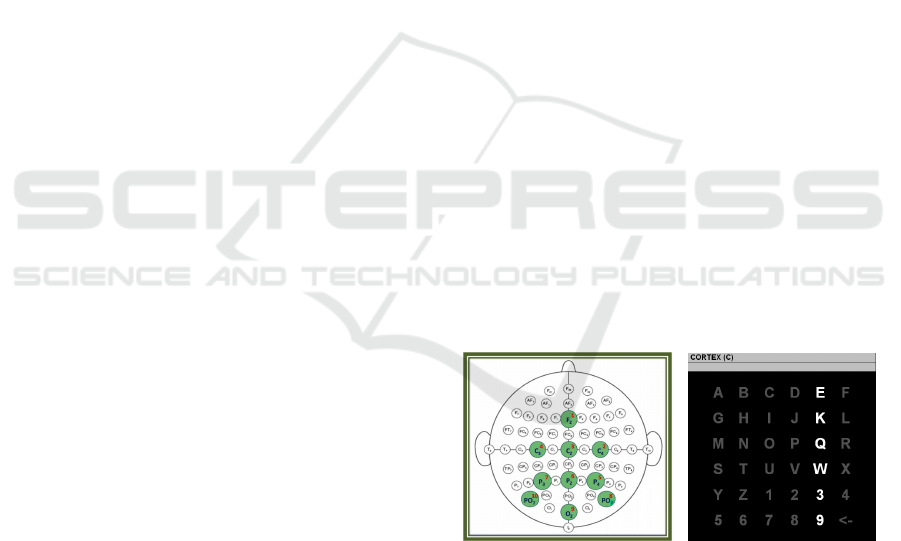
trodes (channels) placed on the scalp (Fig. 1(a)). It

uses an oddball paradigm in which low-probability

target items are inter-mixed with high-probability

non-target items. The speller matrix is usually com-

posed by 36 alphanumeric characters (Fig. 1(b)).

Thus, to spell one character it is necessary to ﬂash

in random order the 6 columns and the 6 rows, while

the user pays attention to the desired letter. When the

letter is highlighted, a P300 is generated by the brain.

The P300 component is a positive deﬂection wave-

form observed around 300 ms after the onset of the

stimulus.

(a) (b)

Figure 1: (a) Location of the 10 recorded EEG channels

used to detect ERP components; (b) A 6x6 P300 speller.

Thus, the task of the P300 speller system is to de-

tect Event-Related Potentials components from the

noisy EEG background signal. It is known to be difﬁ-

cult to accomplish this based on a single trial, because

the magnitude of the EEG background activities is

usually one-order larger than the one of the ERP com-

ponents. Moreover, non-invasive electrodes produce

a noisy signal because the skull dampens signals. So,

the experimental task (single-trial) is repeated many

times and the resulting brain activity is averaged over

trials to increase the signal-to-noise ratio (SNR). This

averaging is made for two reasons: ﬁrst, the ampli-

tude of the ERP waveform is too small to successfully

isolate it from the ongoing EEG activity, and second,

it allows the ﬁltering out of artifacts and noise in the

signal.

However, three major problems with averaging

120

Saavedra C. and Bougrain L..

Wavelet-based Semblance for P300 Single-trial Detection.

DOI: 10.5220/0004191001200125

In Proceedings of the International Conference on Bio-inspired Systems and Signal Processing (BIOSIGNALS-2013), pages 120-125

ISBN: 978-989-8565-36-5

 2013 SCITEPRESS (Science and Technology Publications, Lda.)

ERPs signals are: i) the latency jitter in trials can

smooth out the ERP when averaged, ii) fake ERPs

due to “phase artifacts”, and iii) the communication

bit-rates transfer of the system decreases due to the

number of repetitions required.

For reducing the number of repetitions, it is nec-

essary to develop robust techniques based on stable

features by investigating the time and frequency do-

mains of brain signals.

2 BACKGROUND

There are two techniques commonly used for ERP

feature extraction: “Fisher Spatial Filters” whose

main objective is ﬁnding a linear combination of fea-

tures which characterize or separate classes (Hoff-

mann et al., 2006), and “XDAWN”, which enhance

P300 evoked potentials by using spatial ﬁlters based

on the signal to signal plus noise ratio (Rivet et al.,

2009). Despite the success of these techniques, they

do not consider the available spectral information in

the signal.

Wavelets are very popular for noise ﬁltering of

non-stationary signals. They have being used for

single-trial ERPs detection in several studies (Quiroga

and Garcia, 2003; Yong et al., 2005). The most sui-

table wavelet denoising technique for EEG signals

is the SureShrink (Stein Unbiased Risk Estimator)

(Donoho and Johnstone, 1995), because it ensures the

closest possible reconstruction of the informative sig-

nal, minimizing an estimate of the mean square error.

The problem with these proposed solutions using

wavelets, is that they denoise one channel at a time,

regardless the available information in others cha-

nnels, not considering the information provided by

the ensemble (such as, phase and amplitude infor-

mation). For this reason this paper presents a new

method to denoise EEG signals, which considers the

shared information in the wavelet domain of all cha-

nnels, based on their phase angles correlations. Also,

our algorithm is able to select an appropriate tempo-

ral window for each subject, extracting the interval of

interest to effectively discriminate between classes.

2.1 Wavelets

The Wavelets Transform (WT) is a windowing tech-

nique with variable regions size (Mallat, 2008). The

main idea is to represent a signal x(t) in terms of dis-

placed and shifted versions of a mother wavelet ψ(t),

function:

a,b

(t) = |a|

−



t − b



(1)

where a and b are the scale and translation (time shift)

parameters respectively.

The signal coefﬁcients are obtained by the con-

volution of the original signal x(t) and the different

versions of the mother wavelet :

(a,b) =



x(t)|ψ

a,b

(t)



. (2)

The coefﬁcients refer to the similarity between the

signal and the wavelet at the current scale and time

position. It is possible to distinguish two types of

wavelet analyses depending on values used to com-

pute the scale a and the translation b: the Continuous

Wavelet Transform (CWT), where a and b are con-

tinuous and the Discrete Wavelet Transform (DWT),

where the discrete orthogonal decomposition is ob-

tained using a discretized scale a

= 2

(dyadic step).

The time shift b

is obtained such as that, on a given

scale j + 1, there are twice less coefﬁcients than on

the previous scale.

2.2 Wavelet-based Semblance

Semblance analysis was introduced in Geosciences

by (Cooper and Cowan, 2008) to compare two given

signals x(t) and y(t), using CWT or DWT, based

on phase correlations between the wavelet decom-

positions W

and W

. The ﬁrst step is to compute

the cross-wavelet transform (Torrence and Compo,

1998):

x,y

= W

y∗

(3)

where, ∗ denotes the complex conjugate. The cross-

wavelet amplitude (also called cross-wavelet power)

is given by A = |W

x,y

| and its local phase is deﬁned

as θ = tan

−1

(ℑ(W

x,y

)/ℜ(W

x,y

)), where ℜ and ℑ co-

rrespond to the real and imaginary parts respectively.

The semblance measure S can be used to compare

two signals using θ, deﬁned as:

S = cos

(θ), (4)

where n is an odd integer greater than zero. The

semblance measures the correlations between signals

based on the scale (wavelength)and time (or position)

in the wavelet domain. Its values range from −1 to

1, where S = 1 indicates that signals are correlated ,

S = 0 uncorrelated and S = −1 inversely correlated.

When the mother wavelet is complex, the real and

imaginary parts form a Hilbert transform pair, ensur-

ing orthogonality (Cooper and Cowan, 2008).

As equation 4 does not consider the information of

the amplitude, it is possible to combine the phase in-

formation of S including A as follows:

D = cos

(θ)|W

y∗

|. (5)

This measure can be useful if the signal amplitudes

are important to be analyzed.

Wavelet-basedSemblanceforP300Single-trialDetection

121

2.3 Wavelet Mean Resultant Length

Because the semblance measure is not useful to com-

pare more than two signals, the concept was extended

in (Cooper, 2009) based on circular statistics, by con-

sidering that the beginning and the end of the phases

coincide (0

◦

= 360

◦

). The phases can be treated as

vectors, because the angles denotes a direction (orien-

tation). By connecting all vectors it is possible to ﬁnd

the mean orientation of phases of all signals involved.

If the mean orientation is divided by the number of

vectors used, the Mean Resultant Length (MRL) is

obtained. The MRL can be used as a semblance mea-

sure for more than two signals, which depends of the

number N of signals been treated, so it is possible to

compute it for each time t and scale a:

MRL(t,a) =

(

∑

i=1

ℜ(W

i,t,a

))

+ (

∑

i=1

ℑ(W

i,t,a

))

∑

i=1

i,t,a

(6)

With more than two signals the inversely correlated

concept breaks down, which is veriﬁed by the MRL

values ranging from 0 for uncorrelated signals to 1

for fully correlated signals.

3 METHODS

In this paper we propose to use the Semblance Mea-

sure and the MRL techniques to denoise brain sig-

nals, taking into account the available information of

all recorded channels. This is done by using DWT to

ensure the reconstruction of the original signal. The

choice of DWT is due to its more efﬁcient computa-

tion of the inverse Wavelet Transform than CWT. In

addition, our algorithm have the ability of localizing

the ERP signal in the wavelet domain by selecting an

appropriatetemporal window adapted to each subject,

eliminating non-informative and redundant features.

3.1 Data Denoising

The fundamental hypothesis of wavelet denoising is

that wavelets are correlated with the informative sig-

nal and not correlated with the noise, which globa-

lly means that large coefﬁcients correspond to signal

and small coefﬁcients correspond to noise. There-

fore, noise canceling can be performed by threshold-

ing (Antoniadis, 2007): only large coefﬁcients will

then be used to reconstruct the informative signal.

Let x

(t) be the signal recorded by the c

channel

(or electrode) c ∈ {1, . . .,C} at time t, t ∈ {1,...,T}.

The matrix of recorded EEG signals can be deﬁned as

X ∈ ℜ

TxC

. The MRL is computed using the wavelet

decomposition of all channels W

,∀c through Equa-

tion 6. The MRL coefﬁcients exhibit an exponential

distribution, therefore it is possible to establish a co-

rrelation threshold τ

, based on a logarithmic scale, in

order to set to zero all coefﬁcients that are below the

given threshold. After this process we can reconstruct

the signal using the ﬁltered wavelet coefﬁcients.

The MRL computation is made through the com-

bination of the phase angles of the real and imagi-

nary parts of the wavelet decomposition. DWT uses

wavelets families that are orthogonal to each other, so

the imaginary part can be obtained with the Hilbert

transform of the channel. Algorithm 1 shows the de-

noising process using MRL.

Algorithm 1: MRL Denoising for P300.

Input: Given the EEG signal matrix X contain-

ing C channels and T temporal samples, and the

correlation threshold τ

(e.g., 0.999)

Output: The denoised signals

1: for c = 1 → C do

2: Compute the Hilbert transform H

of x

3: Compute the DWT, W

of signal x

and W

of H

using (2).

4: end for

5: for t = 1 → T do

6: Compute the MRL(t) using (6).

7: if MRL(t) < τ

then

8: set to zero W

at time t, ∀c

9: end if

10: end for

11: for c = 1 → C do

12: Reconstruct the signal for channel c using the

new W

13: end for

3.2 Window Selection

The common procedure in P300 detection is to study

the response during a predeﬁned temporal window af-

ter the stimulus onset. Usually this window corres-

pond to 1 second to be sure to include the P300 re-

sponse and other ERP components in the analysis.

However, the P300 responses have a different latency

and amplitude for each person, causing data to be in-

cluded in the temporal window analysis without been

a relevant inﬂuence in the classiﬁer. We propose to

automatically ﬁnd the temporal window of interest by

detecting where the discriminative information lies to

remove features which do not carry useful informa-

tion. The denoised signal can be denoted by ex

(t),

where c correspond to the channel and t to the instant

BIOSIGNALS2013-InternationalConferenceonBio-inspiredSystemsandSignalProcessing

122

Time After Stimulus (ms)

Scales

0 200 400 600 800 1000

104

112

120

Low

High

(a)

0 200 400 600 800 1000

0.2

0.4

0.6

0.8

Time After Stimulus (ms)

(b)

Figure 2: (a) Dot product D computed using the complex

Morlet wavelet. The colors in the image ranges from blue to

red, and passes through the colors cyan, yellow, and orange

indicating the similarity between GA

and GA

based on

the amplitude and phase information ; (b) Average of D nor-

malized between 0 and 1.

when the signal started to be recorded. Each ex

(t)

has a label to indicate to which class belongs. If we

denote by M the set of all signals, M is composed

by signals belonging to the target class T (containing

a P300 wave) and signals N which are non-targets,

M = {T ,N }. The Grand Averages GA for each class

are computed as:

C|T |

∑

i=1

∑

ex∈T

(t) (7)

C|N |

∑

i=1

∑

ex∈N

(t) (8)

where the operator |.| denotes the cardinal number.

After obtaining the Grand Averages, we compute the

CWT W

and W

to ﬁnally compute the dot

product D through equation 5. The result is shown

in Figure 2(a). Blue color indicates that the signals

have a maximum difference, showing where the P300

is located in the spatial space.

The normalized average avD of D is shown in Fi-

gure 2(b). We can see that the P300 has its center

around 400 ms. Using a threshold τ

, 0 ≤ τ

≤ 1 the

original temporal window of 1s can be reduced to the

interval [t

]. Algorithm 2 describes the window

selection process.

The combination of algorithms 1 & 2 is called the

Denoise and Window Selection MRL model (DWS)

and take the same temporal window for all channels.

A variation on this model is to get a different tem-

poral window for each channel. To do this the only

difference in the process is to compute the average by

channel instead of the grand averages, and do all the

steps for each channel.

4 DATABASE

To validate our method, we used a database ob-

tained from ﬁrst-time users of the P300 speller ap-

plication implemented within the BCI2000 platform

(Schalk et al., 2004). 22 healthy subjects with sim-

ilar characteristics (sleep duration, drugs, age, etc.)

recorded by the Neuroimaging Laboratory of Univer-

sidad Aut´onoma Metropolitana (Mexico) were used.

10 channels, see Figure 1(a), (Fz, C3, Cz, C4, P3,

Pz, P4, PO7, PO8, Oz) have been recorded at 256

sps using the g.tec gUSBamp EEG ampliﬁer, a right

ear reference and a right mastoid ground. An 8th or-

der Chebyshev bandpass ﬁlter, 0.1-60 Hz and a 60 Hz

Notch were used. The stimulus is highlighted for 62.5

ms with an inter-stimuli interval of 125 ms.

A complete description of the parameters used

for the speller and the data are available in

BCI2000 and Matlab formats on the database web-

site: http://akimpech.izt.uam.mx/p300db.

5 EXPERIMENTS

A pre-processing stage were applied to the dataset,

prior to the experiments. The data were ﬁrst ﬁl-

tered by a fourth order forward-backwardButterworth

bandpass ﬁlter. Cut off frequencies were set to 0.1Hz

and 20 Hz (Bougrain et al., 2012). For each cha-

nnel, the bandpass ﬁltered signals were then normali-

zed having zero mean and a standard deviation equal

to one. The temporal window of the post-stimulus re-

sponse was set to 1 s. For XDAWN, we used the pre-

Algorithm 2: Window Selection for P300 Algorithm.

Input: The denoised signals

X and the correla-

tion threshold τ

(e.g. 0.9)

Output: The margins for the temporal window

and t

1: Compute the Grand Averages GA

and GA

signals belonging respectfully to the target class

using (7) and to the non-target class using (8).

2: Compute the CWTs, W

and W

using (2).

3: Compute S, the semblance, using (4) .

4: Compute D using (5).

5: Compute avD, the average of D, and standardize

it between 0 and 1.

6: Compute min(avD), the minimum of avD.

7: Compute the lower boundary t

, the ﬁrst t to the

left of min(avD) which meets AvD(t) > τ

8: Compute the upper boundary t

, the ﬁrst t to the

right of min(avD) which meets AvD(t) > τ

Wavelet-basedSemblanceforP300Single-trialDetection

123

0.4 0.77 1.14 1.51 1.88 2.25 2.62 2.99

−1

−0.5

0.5

1.5

Amplitude (µV)

Time (sec)

original

denoised

Figure 3: Difference between the original signal and its de-

noised version. The shown segment correspond to 3 sec-

onds.

processing presented in (Rivet et al., 2009), to obtain

the best possible result with this technique.

For the experiments, we used a copy spelling se-

ssion and a free spelling session of the database res-

pectively for training and testing a linear support vec-

tor machine (SVM). The datasets contain 5520 reali-

zations for training and 5895 for testing with a time

segment of 1s.

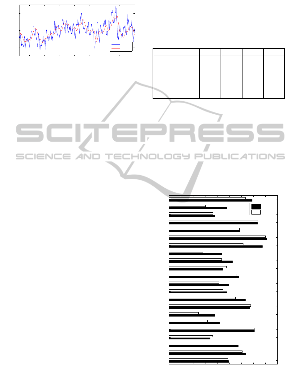
In Figure 3 it is shown the difference between the

original signal and the denoised signal after algorithm

1. We note that the signal is best visualized after de-

noising, making the signal less blurred, what could

improve the study and identiﬁcation of single-trials

responses.

In the ﬁrst experiment we compared ours meth-

ods, DWS

(with the same temporal window for all

channels) and DWS

(with different temporal win-

dows per channel) with the wavelet denoising tech-

nique called VisuShrink and the XDAWN algorithm.

In Table 1 the results for 22 subjects are shown. The

best result is for the proposed algorithms DWS

and

DWS

, proving that the conjoint channel information

is useful to deal with the P300 in single-trial prob-

lem, obtaining better standard deviations. Moreover

as SureShrink and Wavelet-based Semblance are both

part of the wavelet theory it is expected that results

are similar. However, wavelet-based semblance per-

forms signiﬁcatively better. The threshold τ

was set

using the formula 1− τ

= 10

−y

, due to the nature of

the distribution of the MRL coefﬁcients. The thresh-

old was tested for values y = {1,2,3,4}, obtaining the

best result for y = 3.

Due to the different natures of XDAWN and

Wavelet-based Semblance, a more thorough study on

each subject was performed to understand the di-

fferences in the results. In ﬁgure 4 the results by

subject are shown, where Wavelet-based Semblance

shows better performance in 16 subjects over 22. It is

possible to notice that Wavelet-based Semblance and

XDAWN have similar results when the subjects have

high accuracy rates, which suggest that data is cleaner

or the P300 response is stronger making easier the

Table 1: Results obtained using wavelet family Coiﬂet level

3, τ

= 0.999 and τ

= 0.9. The average and the standard

deviation of the letter percentage accuracy over all subjects

and the minimum and maximum accuracy obtained among

subjects are reported. A paired t-test between DWS1 and

XDAWN was signiﬁcant at a 1% level. A paired t-test be-

tween DWS1 and sureShrink was signiﬁcant at a 5% level.

Method mean std min max

None 48.23 15.55 18.10 76.19

XDAWN 51.03 15.80 24.44 80.00

Filter [0.1-20]Hz 53.60 14.14 28.25 79.52

SureShrink 54.80 13.90 33.02 78.57

DWS

55.83 13.49 34.29 80.95

DWS

55.41 13.88 33.97 81.90

classiﬁcation. For subject with poor results, Wavelet-

based Semblance performbetter than XDAWN, there-

fore we conclude that Wavelet-based Semblance per-

forms better in presence of artifacts. DWS

is more

stable among subjects XDAWN allows a data reduc-

tion by selecting the best combinations of signals.

Wavelet-based Semblance achieves a data reduction

selecting a shorter temporal window.

Finally, we compare DWS

and DWS

in Table 2.

The lower and upper boundaries obtained for the new

0 10 20 30 40 50 60 70 80 90

s10

s11

s12

s13

s14

s15

s16

s17

s18

s19

s20

s21

s22

Accuracy in %

Subjects

DWS

XDAWN

Figure 4: Results for the 22 subjects under study for DWS

and XDAWN algorithm.

BIOSIGNALS2013-InternationalConferenceonBio-inspiredSystemsandSignalProcessing

124

temporal window are shown, besides the mean, for all

subjects of the temporal window size.

For DWS

the lower boundary t

was the highest

for subjects 10 and 14, removing approximately 98

ms immediately after the stimulus. This means that

this signal segment does not contain yet enough dis-

criminative information to be useful. For the upper

boundary t

, the lowest value was obtained by sub-

ject 22, removing a little more than half of the original

window, because the window was consider until 488

ms to perform the analysis.

Table 2: Results obtained by DWS

and DWS

on the tem-

poral window selection. t

and t

are respectively the

lower and the higher bounds in ms over all subjects and

channels.

DWS

min 1 1

mean 20 23

max 98 305

min 488 277

mean 848 820

max 1000 1000

Please recall that, for the algorithm DWS

, the

window selected is different for every channel. The

lower boundary t

was the highest for subject 19

in channel 9 (Oz), suggesting that the information

recorded in the ﬁrst 305 ms does not contain enough

discriminative information. The lowest upper bound-

ary t

, obtained for subject 3 at time 277 ms for cha-

nnel 3 (Cz), which is strange because this channel is

usually the one that contains more information. One

explanation is that the electrode is not well-ﬁxed to

the skull or maybe it was moving at the time of the

recording.

6 CONCLUSIONS

Wavelets techniques are becoming an increasingly

important exploration tool in BCI, providing temporal

and spectral information of the signals under study. In

this paper we have introduceda new method to exploit

the correlated information among channels based on

the wavelet-based semblance, measure that was ini-

tially developed to be used in Geosciences. This tech-

nique removes the noise and establishes an appropri-

ate temporal window adapted to each subject. Fur-

thermore, the method is quite general and easy to im-

plement, been possible to be used with others brain

signals.

We empirically demonstrate using the P300

speller application that our method is useful to remove

undesirable component of the signals, improving the

letter accuracy for most of the subjects under study.

One advantage of this method is the ability to adapt to

each subject showing more stability compared with

XDAWN. Also, as the number of features is reduced

by the window selection algorithm, it is likely that the

speed of the classiﬁer may be improved. Despite its

advantages, further studies are needed in order to de-

termine the best threshold parameters.

REFERENCES

Antoniadis, A. (2007). Wavelet methods in statistics: Some

recent developements and their applications. Statistics

Surveys, 1:16–55.

Bougrain, L., Saavedra, C., and Ranta, R. (2012). Finally,

what is the best ﬁlter for p300 detection? Proceedings

of the 3rd TOBI Workshop, pages 53–54.

Cooper, G. (2009). Wavelet-based semblance ﬁltering.

Computers & Geosciences, 35(10):1988–1991.

Cooper, G. and Cowan, D. (2008). Wavelet based sem-

blance analysis. Computers & Geosciences, 34(2):95–

102.

Donoho, D. and Johnstone, I. M. (1995). Adapting to un-

known smoothness via wavelet shrinkage. Journal of

the American Statistical Association, 90:1200–1224.

Farwell, L. and Donchin, E. (1988). Talking off the top of

your head: toward a mental prosthesis utilizing event-

related brain potentials. Electroencephalogr Clin Neu-

rophysiol, 70(6):510–523.

Hoffmann, U., Vesin, J.-M., and Ebrahimi, T. (2006). Spa-

tial ﬁlters for the classiﬁcation of event-related poten-

tials. in Proceedings of the 14th European Symposium

on Artiﬁcial Neural Networks (ESANN).

Mallat, S. (2008). A wavelet tour of signal processing. Aca-

demic Press, 3rd edition.

Quiroga, R. and Garcia, H. (2003). Single-trial event-

related potentials with wavelet denoising. Clinical

Neurophysiology, 114(2):376–390.

Rivet, B., Souloumiac, A., Attina, V., and Gibert, G. (2009).

xdawn algorithm to enhance evoked potentials: Ap-

plication to brain computer interface. IEEE Trans.

Biomed. Engineering, 56(8):2035–2043.

Schalk, G., McFarland, D., Hinterberger, T., Birbaumer, N.,

and Wolpaw, J. (2004). BCI2000: a general-purpose

brain-computer interface (bci) system. IEEE Transac-

tions on Biomedical Engineering, 51(6):1034–1043.

Torrence, C. and Compo, G. (1998). A practical guide to

wavelet analysis. Bulletin of the American Meteoro-

logical Society, 79(1):61–78.

Wolpaw, J., Birbaumer, N., McFarland, D., Pfurtscheller,

G., and Vaughan, T. (2002). Brain-computer inter-

faces for communication and control. Clinical Neuro-

physiology, 113(6):767–791.

Yong, Y., Hurley, N., and Silvestre, G. (2005). Single-trial

EEG classiﬁcation for brain-computer interface using

wavelet decomposition. In European Signal Process-

ing Conference, EUSIPCO 2005.

Wavelet-basedSemblanceforP300Single-trialDetection

125